Articles

You’re a researcher charged with making critical decisions that could impact millions of lives, but you’re blindfolded, left to stumble in the dark.

Sound daunting?

That’s exactly the predicament you face without a firm grasp of sampling distributions and their standard deviations.

These fundamental statistical concepts illuminate the path, transforming educated guesses into accurate inferences and reliable predictions.

Key Highlights

• Learn standard deviation of sampling distributions
• Theoretical foundation
• Intricate calculations
• Step-by-step examples

Sampling Distributions and the Central Limit Theorem

At the heart of statistical analysis lies the concept of sampling distributions – a powerful tool that allows researchers to make accurate inferences about populations based on sample data.

But what exactly are sampling distributions, and how do they relate to the standard deviation of sampling distribution?

A sampling distribution represents the probability distribution of a statistic, such as the sample mean or proportion, calculated from numerous random samples drawn from a population.

In other words, it illustrates the likely variation you’d observe in your statistic if you repeated the sampling process infinitely.

The Central Limit Theorem is a fundamental concept that underpins the use of sampling distributions in statistical inference.

It states that regardless of the population’s distribution shape, the sampling distribution of the mean (standard deviation of sampling distribution of means) approaches a normal distribution as the sample size increases.

This remarkable property allows researchers to rely on the well-known properties of the normal distribution, even when the population is not normally distributed.

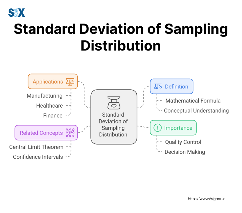
Distinguishing Population, Sample, and Sampling Distribution Statistics

Before we dive deeper, it’s crucial to understand the distinctions between population parameters, sample statistics, and sampling distribution statistics:

• Population parameters: These are fixed values that describe the entire population, such as the population mean (μ) and the population standard deviation (σ).
• Sample statistics: These are calculated values based on a sample drawn from the population, such as the sample mean (x̄) and the sample standard deviation (s). They serve as estimates of the corresponding population parameters.
• Sampling distribution statistics: These describe the probability distribution of a statistic calculated from numerous samples, such as the mean (standard deviation of sampling distribution) and the standard error of the mean.

For example, let’s consider a population of test scores with a mean of 75 and a standard deviation of 10.

If we draw a sample of 30 scores, we might calculate a sample mean of 77 and a sample standard deviation of 8.

However, if we repeated this sampling process numerous times, we’d obtain a range of sample means, and their distribution would follow the sampling distribution of the mean, with a mean of 75 (the population mean) and a standard deviation of 10/√30 ≈ 1.83 (the standard deviation of sampling distribution).

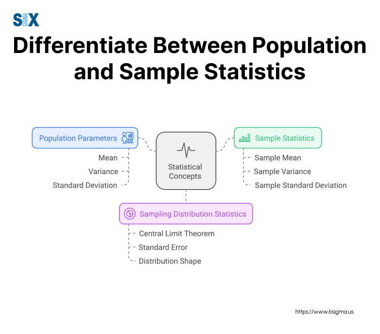
The Journey from Sample to Sampling Distribution

To better grasp the concept of sampling distributions, let’s walk through the process of generating one:

1. Define the population and the statistic of interest (e.g., mean, proportion).
2. Draw a random sample from the population and calculate the statistic.
3. Plot the statistic’s value on a histogram or density curve.
4. Repeat steps 2 and 3 numerous times (ideally, tens of thousands of times) with different random samples.

As you repeat this process, the histogram will gradually take the shape of the sampling distribution for that statistic. Interactive simulations can be powerful tools to visualize this process and build an intuitive understanding.

It’s important to note that while individual samples may vary, the sampling distribution itself has a predictable shape, mean, and standard deviation, governed by the Central Limit Theorem.

This consistency is what allows researchers to make reliable inferences about populations based on sample data.

However, some common misconceptions can arise, such as confusing the sampling distribution with the population distribution or assuming that all sampling distributions are normal. Addressing these potential sources of confusion is crucial for a solid grasp of the concept.

Ready to unlock the power of data-driven decision-making? Our Yellow Belt course equips you with essential tools to understand and leverage sampling distributions for accurate statistical analysis.

Mastering the Calculations of Sampling Distributions: Formulas and Step-by-Step Examples

While the conceptual understanding of sampling distributions is crucial, mastering the calculations is equally vital for accurate statistical analyses.

The formula for calculating the standard deviation of the sampling distribution is remarkably simple:

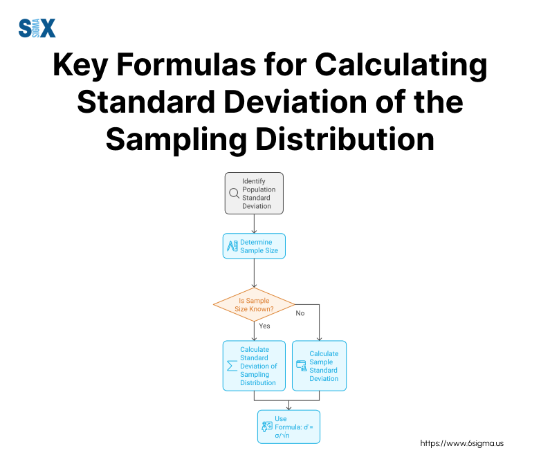
Standard Deviation of Sampling Distribution = Population Standard Deviation / √Sample Size
σ = σ / √n

Where:
σ = Standard deviation of the sampling distribution
σ = Population standard deviation
n = Sample size

Let’s illustrate this with an example:

Suppose we’re studying the heights of adult males in a certain population, which follows a normal distribution with a mean of 175 cm and a standard deviation of 8 cm.

If we draw a random sample of 50 individuals, how to calculate the standard deviation of sampling distribution?

Given:
Population standard deviation (σ) = 8 cm
Sample size (n) = 50

Plugging these values into the formula:
σ = σ / √n
= 8 / √50
= 8 / 7.07
= 1.13 cm

Therefore, the standard deviation of the sampling distribution of means for samples of size 50 is approximately 1.13 cm.

A few expert tips to keep in mind when calculating the standard deviation of sampling distribution:

1. Ensure you’re using the population standard deviation (σ), not the sample standard deviation (s).
2. For small sample sizes, be cautious about assuming normality in the sampling distribution.
3. Double-check your units to avoid common calculation errors.

Simplifying Complex Scenarios with the Standard Deviation of Sampling Distribution

While the formula works well for many situations, it’s essential to consider alternative approaches for non-normal populations or finite population adjustments.

For example, when dealing with non-normal distributions, you may need to rely on resampling techniques like bootstrapping to estimate the sampling distribution’s standard deviation. We’ll explore these advanced methods in a later section.

In finite populations, where the sample size is a significant proportion of the population, an adjustment factor is applied to account for the reduced variance. The adjusted formula becomes:

Standard Deviation of Sampling Distribution = √[(N – n) / (N – 1)] * (σ / √n)

Where N is the population size.

Selecting the appropriate technique depends on factors like population distribution, sample size, and the nature of your data. We’ll provide guidance on navigating these complexities to ensure accurate and reliable results.

Interactive Exploration

To solidify your understanding, let’s put theory into practice with an interactive simulation.

This tool allows you to input various population parameters, sample sizes, and distribution types, visualizing the resulting sampling distribution in real-time.

As you experiment with different scenarios, pay close attention to how changes in sample size, population variance, and distribution shape impact the standard deviation of the sampling distribution.

This hands-on exploration will not only reinforce conceptual mastery but also prepare you for practical applications in research or business settings.

With a solid grasp of the calculations, formulas, and the ability to navigate complex scenarios, you’ll be well-equipped to harness the power of the standard deviation of sampling distribution in your statistical analyses.

Take your data analysis skills to the next level. Learn to apply powerful statistical tools and master advanced sampling distribution calculations in our comprehensive Green Belt program.

Applications in Statistical Inference: Confidence Intervals and Hypothesis Testing

While mastering the calculations is crucial, the true power of the standard deviation of sampling distribution lies in its applications for robust statistical inference.

This measure plays a pivotal role in constructing confidence intervals and conducting hypothesis tests – two fundamental techniques that allow researchers to draw reliable conclusions from their data.

Confidence intervals provide a range of values within which the true population parameter is likely to fall, based on the sample data.

The standard deviation of sampling distribution is an essential component in determining the interval’s width, ensuring an appropriate level of precision and confidence.

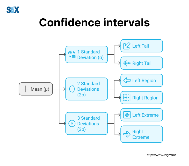
For example, let’s construct a 95% confidence interval for the mean height of adult males in a population, using a sample of 50 individuals with a mean height of 178 cm and a known population standard deviation of 8 cm.

Given:
Sample mean (x̄) = 178 cm
Population standard deviation (σ) = 8 cm
Sample size (n) = 50
Confidence level = 95%

First, we calculate the standard deviation of the sampling distribution:
σ = σ / √n
= 8 / √50
= 1.13 cm

Next, we find the critical value (z) for a 95% confidence level from the standard normal distribution table (z = 1.96).

The confidence interval is then calculated as:
x̄ ± z*(σ)
178 cm ± (1.96 × 1.13 cm)
= 178 cm ± 2.21 cm
= (175.79 cm, 180.21 cm)

We can interpret this result as: “We are 95% confident that the true mean height of adult males in the population lies between 175.79 cm and 180.21 cm”.

In addition to confidence intervals, the standard deviation of sampling distribution is instrumental in hypothesis testing, where researchers assess the plausibility of a specific claim or hypothesis about a population parameter.

By comparing the sample statistic to the hypothesized value and considering the sampling distribution’s variability, researchers can determine the likelihood of observing such a result if the hypothesis is true.

Tailored Examples of Standard Deviation of Sampling Distribution from Multiple Disciplines

The applications of the standard deviation of sampling distribution extend across diverse fields, each with its unique challenges and contexts.

In business settings, it plays a crucial role in market research, customer segmentation, and quality control processes.

For instance, determining the sample size required to estimate consumer preferences within a specific margin of error or assessing whether a product meets quality standards based on a sample inspection.

Scientific studies, such as experimental design, survey analysis, and clinical trials, heavily rely on the standard deviation of sampling distribution.

Researchers calculate confidence intervals for treatment effects, test hypotheses about drug efficacy, and ensure adequate statistical power to detect meaningful differences.

Social science research also benefits from a deep understanding of this concept.

Opinion polls, behavioral studies, and policy evaluations all involve drawing inferences from sample data, where the standard deviation of sampling distribution guides researchers in making statistically sound conclusions.

Throughout these examples, we’ll leverage real-world datasets to illustrate the concepts, ensuring a grounded and practical understanding of the applications.

Expert Insights on Best Practices for Standard Deviation of Sampling Distribution

While the formulas and techniques are well-established, their effective application often requires nuanced considerations and expert guidance.

From selecting appropriate methods based on study objectives and constraints to interpreting and communicating results effectively, these expert perspectives will equip you with the knowledge and skills necessary to navigate the complexities of statistical inference with confidence.

Become a statistical analysis expert with our Black Belt course prepares you to lead organization-wide data initiatives and drive strategic excellence through advanced statistical techniques like sampling distributions.

Exploring the Cutting Edge: Advanced Techniques and Emerging Trends

While the traditional methods for calculating and applying the standard deviation of sampling distribution remain invaluable, the field of statistics is constantly evolving, with researchers exploring new frontiers and pushing the boundaries of what’s possible.

One such technique is bootstrapping, a powerful resampling method that allows researchers to approximate the sampling distribution without making assumptions about the underlying population distribution.

By repeatedly drawing samples with replacement from the original dataset, bootstrapping simulates the process of repeated sampling, providing estimates of the standard deviation of sampling distribution and other statistics.

For example, in a study investigating the effectiveness of a new marketing campaign, researchers could use bootstrapping to estimate the sampling distribution of the difference in conversion rates between the treatment and control groups, without assuming normality or relying on asymptotic theory.

Another exciting development in the realm of sampling distributions is the integration of Bayesian approaches.

Unlike the traditional frequentist methods, Bayesian statistics treat parameters as random variables and incorporate prior knowledge or beliefs into the analysis.

This paradigm shift opens up new avenues for modeling complex sampling distributions, particularly in scenarios with limited data or hierarchical structures.

The field of sampling distributions is also benefiting from advancements in computational power and machine learning techniques.

Researchers are exploring the use of neural networks and other AI models to approximate sampling distributions, potentially enabling more accurate and efficient analyses, even for high-dimensional or non-standard scenarios.

Interactive Simulation of Sampling Distributions

To provide a hands-on experience with these cutting-edge techniques, we’ve developed an interactive simulation that allows you to experiment with bootstrapping and Bayesian methods for estimating sampling distributions.

This tool not only visualizes the results but also compares them to traditional methods, highlighting the trade-offs and potential advantages of each approach.

As you explore these advanced techniques, pay close attention to the assumptions, data requirements, and computational considerations involved.

While they offer exciting new possibilities, it’s crucial to understand their limitations and appropriate use cases to ensure reliable and meaningful results.

The future of sampling distributions is undoubtedly bright, with ongoing research and development promising even more powerful tools and insights for statistical analysis.

By staying abreast of these emerging trends and embracing new techniques, you’ll be well-positioned to tackle complex problems and drive innovation in your field.

Conclusion

In this comprehensive guide, we’ve explored the foundations of sampling distributions, mastered the calculations of their standard deviations, and delved into their pivotal applications in statistical inference.

From constructing confidence intervals to conducting hypothesis tests, the standard deviation of sampling distribution has proven to be an indispensable tool for researchers and professionals across various domains.

Moreover, we’ve looked ahead to the cutting edge of the field, introducing advanced techniques like bootstrapping and Bayesian methods, as well as emerging trends that promise to shape the future of sampling distributions.

So, whether you’re a student grappling with complex formulas, a researcher pushing the boundaries of knowledge, or a professional seeking to enhance your analytical skills, this guide has equipped you with the tools and insights necessary to harness the full power of the standard deviation of sampling distribution.

We encourage you to apply the knowledge you’ve gained, experiment with the interactive tools and simulations, and continue exploring the vast realm of sampling distributions.

Remember, the path to statistical enlightenment is an ongoing journey, and with the right resources and dedication, you can unlock new frontiers of understanding and innovation.

If you found this guide valuable, we invite you to explore our other resources, including online courses, webinars, and consulting services, where you can further deepen your expertise in statistics and data analysis.

Stay curious, keep learning, and let the standard deviation of sampling distribution be your guide to making data-driven decisions that drive real-world impact.