Articles

Standard deviation of residuals is a cornerstone in regression analysis and model evaluation, providing invaluable insights into the accuracy and reliability of our predictive models.

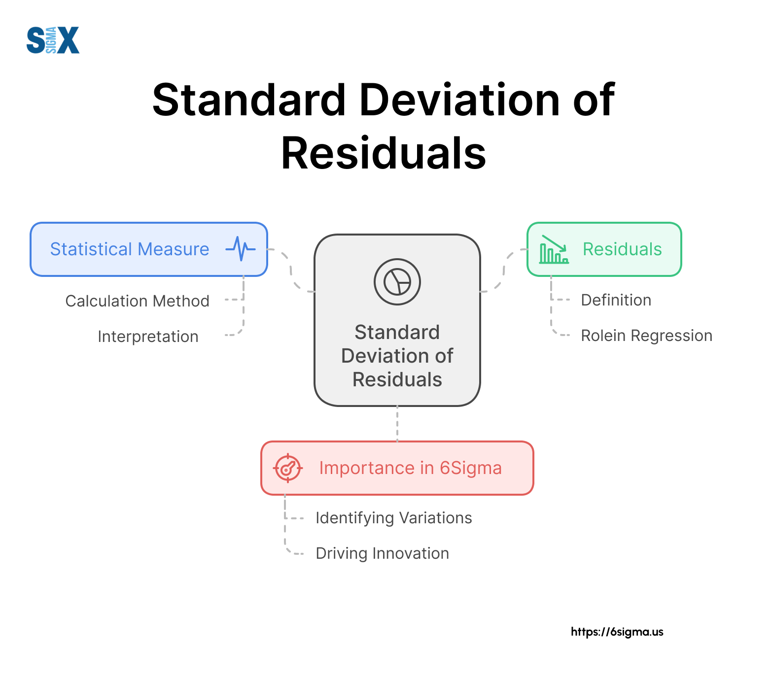
The standard deviation of residuals, often denoted as S or Sy.x, quantifies the typical vertical distance between observed data points and the fitted regression line or curve.

It’s a powerful tool in our statistical arsenal, allowing us to assess the goodness-of-fit of our models and make informed decisions in various industrial and business contexts.

Understanding these statistical concepts is crucial for professionals pursuing Six Sigma certification, as they form the foundation of data-driven decision-making in process improvement across industrial and business settings.

Key Highlights

• Definition and significance in statistical modeling
• Residuals: Observed vs. predicted values in regression
• Step-by-step calculation process and formula explanation
• Applications in model accuracy and outlier detection
• Advanced concepts: Heteroscedasticity and robust regression
• Practical interpretation and decision-making implications

Introduction to Standard Deviation of Residuals

Standard deviation of residuals is a critical concept in statistical modeling.

It’s a measure that quantifies the typical difference between observed data points and the values predicted by our regression model.

This metric is essential for assessing how well our model fits the data and for making reliable predictions. Professionals with a six sigma certification are often trained to leverage metrics like this for process optimization and error reduction in industrial settings.

The standard deviation of residuals, often denoted as S or Sy.x, is calculated using the residuals from our regression analysis.

These residuals are the vertical distances between our observed data points and the fitted regression line or curve.

By analyzing these residuals, we gain valuable insights into the accuracy and reliability of our statistical models.

Relationship to Regression Analysis and Goodness-of-fit

In regression analysis, our goal is to find the best-fitting line or curve that describes the relationship between our variables.

The standard deviation of residuals plays a crucial role in determining the goodness-of-fit of our model.

A smaller standard deviation indicates that our data points are closer to the regression line, suggesting a better fit.

This measure is closely related to other goodness-of-fit statistics, such as R-squared.

However, while R-squared tells us the proportion of variance explained by our model, the standard deviation of residuals provides a more tangible measure of the typical deviation of our data points from the model predictions. Understanding this distinction is crucial for practical application, a key learning outcome for those pursuing Six Sigma Green Belt certification.

Understanding Standard Deviation of Residuals in Regression Analysis

Residuals are the foundation of model assessment in regression analysis.

For those pursuing a Six Sigma certification, mastering the concept of residuals is essential, as it’s a building block for the statistical techniques used to optimize processes.

Concept of Observed Values vs. Predicted Values

In my work with companies like 3M and Intel, I’ve often emphasized the importance of understanding the difference between observed and predicted values.

Observed values are the actual data points we collect, while predicted values are those generated by our regression model.

The discrepancy between these two sets of values forms the basis of our residual analysis.

Calculating Standard Deviation of Residuals and their Interpretation

Residuals are calculated by subtracting the predicted value from the observed value for each data point.

A positive residual indicates that our model underestimated the observed value, while a negative residual suggests an overestimation.

The magnitude of these residuals gives us insight into how well our model is performing across different regions of our data.

Residual Plots and their Significance

Residual plots are powerful diagnostic tools that I’ve used extensively in my statistical process control work.

These plots help us visualize patterns in our residuals, which can reveal important information about our model’s adequacy. Interpreting these plots effectively is a vital diagnostic skill, particularly emphasized in Six Sigma Black Belt certification where complex process analysis is common.

A well-fitted model should produce residuals that are randomly scattered around zero with no discernible pattern.

Calculating the Standard Deviation of Residuals

The standard deviation of residuals quantifies the typical spread of data points around the regression line.

Formula and Step-by-step Process

The formula for the standard deviation of residuals is:

S = √[Σ(yi – ŷi)² / (n – p)]

Where:

• yi are the observed values
• ŷi are the predicted values
• n is the number of observations
• p is the number of parameters in the model

To calculate this:

1. Compute the residuals (yi – ŷi) for each data point
2. Square these residuals
3. Sum the squared residuals
4. Divide by (n – p)
5. Take the square root of the result

This calculation is a basic skill introduced in Six Sigma Yellow Belt certification programs, where professionals start exploring statistical tools for process improvement.

Comparison of Standard Deviation of Residuals with Root Mean Square Error (RMSE)

The standard deviation of residuals is closely related to the root mean square error (RMSE). In fact, for simple linear regression, they are identical.

However, for multiple regression or more complex models, this accounts for the number of parameters in the model, making it a more appropriate measure of model fit.

Interpreting the Standard Deviation of Residuals

In my experience working with various industries, I’ve found that interpreting the standard deviation of residuals requires context.

Generally, a smaller value indicates a better fit, but what constitutes “small” depends on the scale of your data and the specific application.

It’s often useful to compare this value to the overall variability in your dependent variable to gauge the model’s predictive power.

Learn the detailed calculation process for the standard deviation of residuals to implement advance data techniques with our Lean Six Sigma Green Belt Certification and Training Program

Applications of Standard Deviation of Residuals

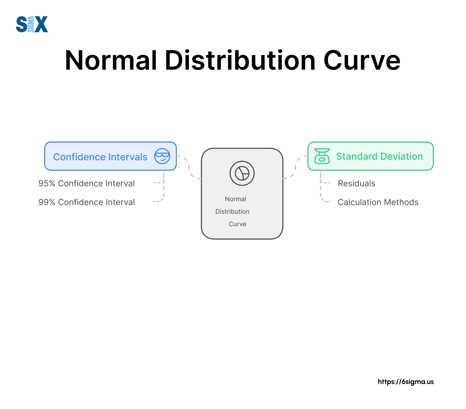
This measure is invaluable for assessing model accuracy, identifying outliers, and constructing confidence intervals.

Professionals with a Six Sigma Green Belt certification often rely on these techniques to analyze data and optimize processes in real-world projects.

Assessing Model Accuracy and Predictive Power

The standard deviation of residuals is a key metric for assessing how well our model can predict new observations.

In my work with companies like GE and HP, we’ve used this measure to compare different models and select the one with the best predictive power for the task at hand.

Identifying Outliers and Influential Data Points with Standard Deviation of Residuals

By examining residuals that are several standard deviations away from zero, we can identify potential outliers or influential points.

This process has been crucial in my experience with mixture experimentation and design of experiments, where unusual observations can significantly impact our conclusions.

Spotting outliers is a key step in analyzing root causes, a skill emphasized in Six Sigma methodology and often taught in root cause analysis training.

Use in Hypothesis Testing and Confidence Intervals

It plays a vital role in constructing confidence intervals for our regression coefficients and predictions.

It’s also used in hypothesis tests to determine the statistical significance of our model parameters, a crucial step in ensuring the reliability of our statistical inferences.

Advanced Concepts in Residual Analysis

Advanced residual analysis involves dealing with heteroscedasticity, employing robust regression techniques, and adapting to nonlinear relationships.

Heteroscedasticity and its Impact on Residuals

Heteroscedasticity, a condition where the variability of residuals is not constant across all levels of the independent variables, can significantly impact our model’s validity.

These advanced techniques, like handling heteroscedasticity, are often covered in Six Sigma Black Belt certification programs, where practitioners tackle complex data challenges.

In my work with complex manufacturing processes, I’ve often encountered this issue and developed strategies to detect and address it, such as using weighted least squares regression.

Robust Regression Techniques for Handling Outliers with Standard Deviation of Residuals

When deal ing with datasets that contain outliers or influential points, robust regression techniques can be invaluable.

These methods, which I’ve applied in various industrial settings, aim to produce reliable estimates even in the presence of extreme observations, often requiring the advanced statistical toolkit associated with Six Sigma Black Belt certification.

Nonlinear Regression and Residual Standard Error

In many real-world applications, particularly in chemical engineering and product development, relationships between variables are often nonlinear.

In these cases, we need to adapt our approach to residual analysis, using techniques like the residual standard error to assess the fit of our nonlinear models.

Know some advanced concepts in residual analysis with Statistical Process Control

Conclusion

From its calculation and interpretation to its applications in model assessment and advanced analysis techniques, this metric provides invaluable insights into the quality and reliability of our regression models.

It is more than just a number – it’s a key to understanding the uncertainty in our predictions and the overall performance of our models.

As we’ve seen, it plays a critical role in hypothesis testing, confidence interval construction, and model comparison.

As statistical modeling advances, integrating the fundamentals of Lean with Six Sigma will be key to driving efficiency and quality in future process improvements.

Future Trends in Residual Analysis and Statistical Modeling

Looking ahead, I anticipate that residual analysis will continue to evolve, particularly in the realm of big data and machine learning.

Combining residual analysis with lean fundamentals—emphasizing waste reduction and efficiency—can create powerful frameworks for data-driven decision-making

We’re likely to see new techniques for handling complex, high-dimensional datasets and more sophisticated methods for visualizing and interpreting residuals in these contexts.

As statisticians and data scientists, our ability to effectively use tools like the standard deviation of residuals will remain crucial in extracting meaningful insights from data and driving data-informed decision-making across industries.