Articles

Regression analysis proves a potent statistical technique relating outcome variables to one or more influence variables.

However, models heavily rely on sound foundations and quality information. Here residual examination plays an essential role in assumptions evaluation and fit adequacy assessment.

Residuals describe gaps between observed outcome values and those predicted.

Containing valuable clues about performance, residuals may reveal assumption breaches or systematic patterns demanding further review or remedies.

Residual analysis involves comprehensive residue examination through graphical and numerical methods.

Analyzing residues assists researchers and analysts in pinpointing concerns including non-linearity, uneven variance, interdependence, impactful observations, and outliers.

Addressing such concerns ensures model validity, resilience, and enhanced prediction/inference capabilities – crucial for drawing meaningful conclusions.

For continual problem-solvers committed to understanding nature’s interconnected dances through numbers, residual analysis emerges as a trusted partner.

Key Highlights

• Residual analysis is a crucial diagnostic technique in regression analysis to evaluate the validity of model assumptions and assess the adequacy of the fitted model.
• It involves examining the residuals, which are the differences between the observed values and the predicted values from the regression model.
• Residual plots and patterns provide valuable insights into potential violations of model assumptions, such as non-linearity, heteroscedasticity, and autocorrelation.
• Identifying outliers and influential observations through residual analysis is essential to ensure the robustness and reliability of the model.
• Residual analysis methods, including studentized residuals, Cook’s distance, DFFITS, and DFBETAS, aid in detecting and handling influential data points.
• Techniques like partial residual plots, added variable plots and scale-location plots assist in diagnosing specific model inadequacies and potential remedies.
• Residual transformations and weighted least squares regression can address issues like non-constant variance and improve model fit.

Introduction to Residual Analysis

Residual analysis is a crucial step in assessing the validity and adequacy of a regression model.

A residual is the difference between an observed value and the value predicted by the regression model.

Analyzing these residuals provides valuable insights into whether the key assumptions of the regression model are met, and helps identify any violations or potential issues with the model.

The primary goal of the residual analysis is to validate the regression model’s assumptions, such as linearity, normality, homoscedasticity (constant variance), and independence of errors.

If these assumptions are violated, the regression results may be unreliable or misleading, necessitating remedial measures or alternative modeling approaches.

Residual analysis involves a series of diagnostic techniques and graphical methods to examine the behavior and patterns of residuals.

These include residual plots, tests for normality, heteroscedasticity detection, outlier identification, and assessments of influential observations.

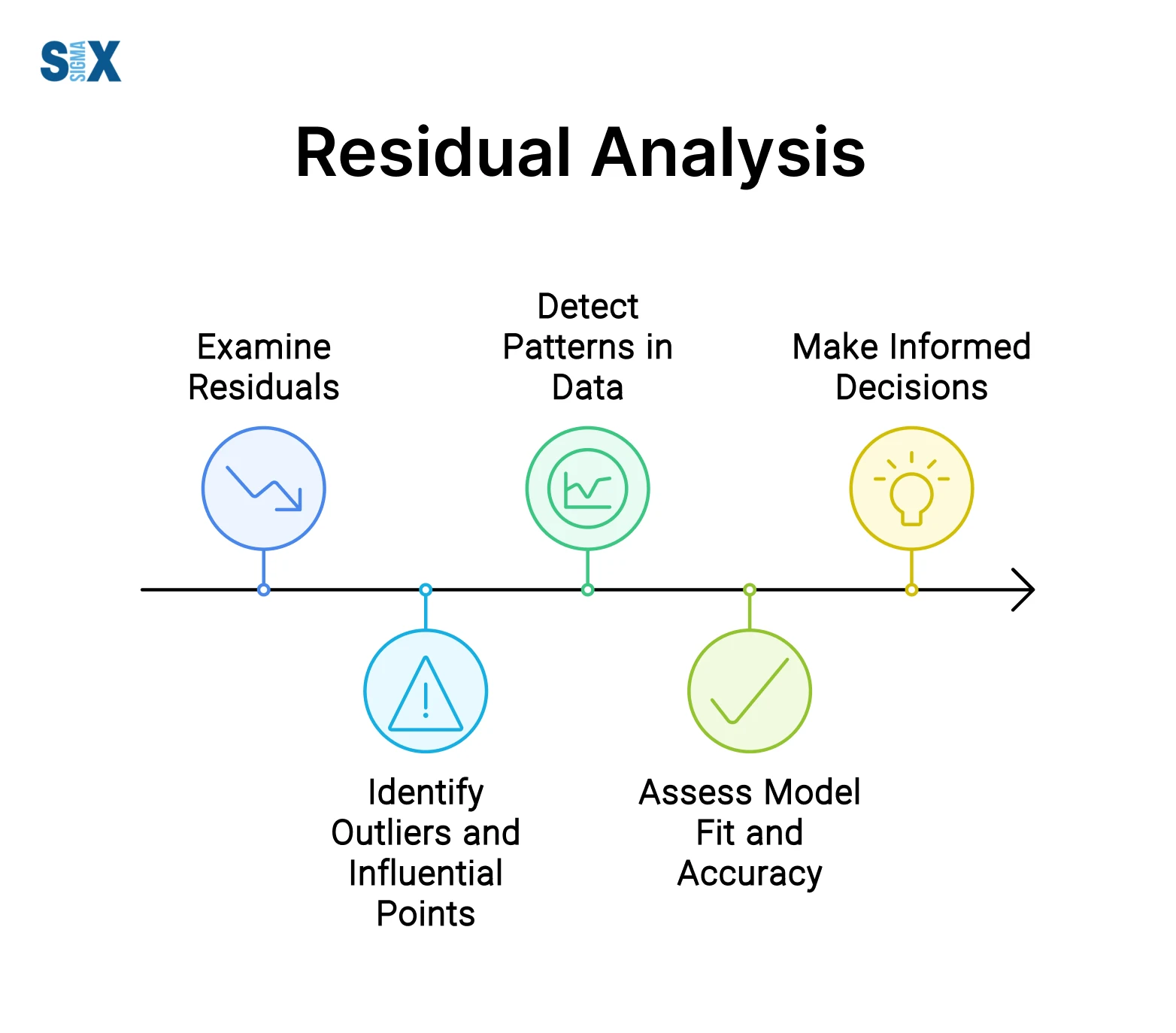
By carefully scrutinizing the residuals, analysts can gain a deeper understanding of the model’s fit, identify potential sources of bias or inefficiency, and make informed decisions about the appropriateness of the regression model.

Conducting a thorough residual analysis is an essential step in the regression modeling process, as it helps ensure the validity and reliability of the model’s predictions and inferences.

Deepen your understanding of statistical analysis and graphical techniques. Introduction to Statistics and Graphical Analysis course provides a solid foundation to master residual analysis and key statistical concepts.

It is a critical component of model validation techniques and regression diagnostics, enabling researchers and analysts to have greater confidence in their analytical results and decision-making processes.

Residual Plots and Patterns

Residual plots are a powerful diagnostic tool for visualizing the residuals from a regression model.

By examining the patterns in residual plots, analysts can assess whether the key assumptions of the regression model have been violated. Several common residual plots are used in the residual analysis:

Residuals vs Fitted Values Plot

This plot shows the residuals on the vertical axis against the fitted values (predicted values from the model) on the horizontal axis. Ideally, the residuals should be randomly scattered around the horizontal line representing zero.

Any pattern or shape in this plot violates the linearity or homoscedasticity assumptions.

Residuals vs Predictor Variable Plots 

These plots display the residuals against each predictor variable in the model. Again, the residuals should appear randomly scattered with no discernible pattern.

Curved or funnel shapes can signify non-linear relationships or heteroscedasticity.

Normal Q-Q Plot within Residual Analysis

A normal Q-Q plot assesses whether the residuals follow a normal distribution by plotting their quantiles against theoretical quantiles from a normal distribution.

Points should closely follow the 45-degree reference line for the residuals to be normally distributed.

Scale-Location Plot

This plot shows the square root of the absolute residuals versus the fitted values to check for heteroscedasticity.

A random scatter indicates constant variance, while a funnel shape implies heteroscedasticity.

Recognizing Residual Patterns with Residual Analysis

Some common patterns in residual plots can provide clues about violations of regression assumptions:

• Funneling pattern: Indicates heteroscedasticity (non-constant variance)
• Curved shape: Suggests non-linear relationship between predictor and response
• Shifted/skewed pattern: May indicate outliers or influential observations
• Cyclic pattern: Points to autocorrelation or time-based effects
• By carefully examining residual plots and identifying any systematic patterns, analysts can determine whether the regression model assumptions are met or if remedial measures are needed.

Create and interpret these residual plots yourself! Introduction to Graphical Analysis with Minitab course offers hands-on training in creating and analyzing statistical plots.

Assessing Model Assumptions with Residual Analysis

One of the primary purposes of residual analysis is to check whether the key assumptions of the regression model are violated.

These assumptions are crucial for the model to provide reliable and unbiased estimates. By examining the residual patterns, we can assess the validity of these assumptions.

Normality Assumption

The normality assumption states that the residuals should follow a normal distribution. A violation of this assumption can lead to invalid statistical inferences.

To assess normality, we can use residual quantile plots or normal probability plots.

These plots compare the quantiles of the residuals against the quantiles of a normal distribution.

If the points deviate substantially from the reference line, it may indicate a violation of the normality assumption.

Residual Independence

The residuals should be independent, meaning that the residual values are not correlated with each other.

Autocorrelation in the residuals can arise due to temporal effects or omitted variables. We can check for residual independence using the Durbin-Watson test or by examining residual autocorrelation plots.

These plots display the residuals against their lagged values, and any patterns or trends may suggest a violation of the independence assumption.

Constant Variance (Homoscedasticity) with Residual Analysis

The residuals should have constant variance across all levels of the predictor variables.

Heteroscedasticity, or non-constant variance, can lead to inefficient parameter estimates and invalid confidence intervals.

To detect heteroscedasticity, we can use residual vs. fitted value plots or scale-location plots.

These plots display the residuals against the fitted values or a predictor variable. If the spread of the residuals varies systematically across the range of values, it may indicate heteroscedasticity.

Linearity Assumption

For linear regression models, the relationship between the response variable and the predictor variables should be linear.

Non-linear patterns in the residuals may suggest a violation of this assumption.

Partial residual plots and added variable plots can help identify non-linear relationships. These plots display the residuals against a predictor variable after accounting for the effects of other predictors.

By carefully examining the residual patterns and conducting appropriate statistical tests, we can assess whether the model assumptions are met.

If violations are detected, appropriate remedial measures, such as data transformations or alternative modeling techniques, may be necessary to ensure the validity and reliability of the regression analysis.

Identifying Outliers and Influential Observations with Residual Analysis

Outliers and influential observations can have a major impact on the results of a regression analysis.

Residual analysis provides several diagnostic tools to detect these problematic data points.

Outliers are observations that deviate substantially from the overall pattern of the other data points.

They can arise from measurement errors, data entry mistakes, or simply unusual events.

Outliers can severely bias the regression coefficients and inflate the residual variance, reducing the predictive ability of the model.

Several residual statistics help flag potential outliers:

• Studentized Residuals: Standardized residuals that are corrected for the effect of deleting the observation. Large absolute values (e.g. >3) indicate possible outliers.
• Leverage: Measures how far an observation is from the mean predictor values. High leverage points (e.g. >2p/n where p is the number of predictors) can potentially be outliers or influential points.  

In addition to outliers, influential observations are data points that have an excessive impact on the regression results.

They may not appear as obvious outliers, but deleting them would significantly change the estimated coefficients.

Common measures of influence include:

• Cook’s Distance: This shows how much deleting an observation would change the fitted values for all other observations. Large values (e.g. >4/n) indicate influence.
• DFFITS: Measures the number of standard error movements an observation would cause in the predicted values if deleted. The cutoff depends on the significance level.
• DFBETAS: The standardized change in each coefficient if the observation is deleted. Values >2/sqrt(n) suggest influence.
• Partial residual plots and added variable plots can also help visualize outliers and influential points. Observations with high leverage and large residuals are clear candidates for further investigation and potential elimination from the dataset.

Properly identifying and handling outliers and influential observations through residual diagnostics is crucial for obtaining reliable regression results and valid statistical inferences.

Detecting Heteroscedasticity

One of the key assumptions of linear regression is homoscedasticity, which means the residuals should have constant variance across all levels of the predictor variables.

Violation of this assumption, known as heteroscedasticity, can lead to inefficient parameter estimates and invalid inference. Therefore, detecting heteroscedasticity is an important step in residual analysis.

Residual Plots for Heteroscedasticity Detection

The most common approach to detect heteroscedasticity is to visually inspect residual plots. Some useful residual plots include:

Residuals vs Fitted Values Plot: This plot shows the residuals on the y-axis and the fitted/predicted values on the x-axis.

If the residuals are randomly scattered with no systematic pattern, it suggests homoscedasticity.

However, if the residuals exhibit a funnel shape or their spread increases/decreases as the fitted values increase, it indicates heteroscedasticity.

Scale-Location Plot: This plot shows the square root of the absolute residuals on the y-axis and the fitted values on the x-axis.

Similar to the previous plot, a random scatter suggests homoscedasticity, while an increasing/decreasing trend implies heteroscedasticity.

Residuals vs Predictor Plots: These plots show the residuals on the y-axis and each predictor variable on the x-axis. Any systematic pattern or unequal spread of residuals across the range of predictor values can indicate heteroscedasticity.

Statistical Tests for Heteroscedasticity

In addition to graphical methods, there are several statistical tests to formally detect heteroscedasticity, such as:

Breusch-Pagan Test: This test examines the relationship between the squared residuals and the predictor variables.

A significant test result indicates the presence of heteroscedasticity.

White’s Test: Similar to the Breusch-Pagan test, but it includes additional terms involving cross-products of the predictors, making it more general.

Goldfeld-Quandt Test: This test divides the data into two groups based on the values of a predictor variable and compares the residual variances between the two groups.

Glejser Test: This test regresses the absolute residuals on the predictor variables and checks if the coefficients are significantly different from zero, which would indicate heteroscedasticity.

Dealing with Heteroscedasticity

If heteroscedasticity is detected, several remedial measures can be taken, such as:

• Weighted Least Squares (WLS) regression, which assigns different weights to observations based on their variance.
• Transformations of the response variable or predictor variables to stabilize the variance.
• Including additional predictor variables or interaction terms in the model to account for the heteroscedasticity.
• Robust standard errors that are valid under heteroscedasticity.

By detecting and addressing heteroscedasticity, residual analysis helps ensure the validity and efficiency of the regression model.

Multicollinearity and Residual Analysis

Multicollinearity refers to the situation where two or more predictor variables in a regression model are highly correlated with each other.

This can cause issues in interpreting the individual effects of each variable and can lead to unstable estimates of the regression coefficients.

Residual analysis can help detect the presence of multicollinearity in a regression model.

One way to identify multicollinearity through residual analysis is to examine the residual patterns.

If there are distinct patterns or structures in the residual plots, it may indicate that the model is missing important predictor variables or that there are interactions between variables that need to be accounted for.

These patterns can sometimes arise due to multicollinearity.

Another approach is to look at influence statistics like DFBETAS, which measures the change in a regression coefficient when a particular observation is deleted.

Large values of DFBETAS for one or more predictors can signal multicollinearity issues. Examining partial residual plots and added variable plots can also reveal potential multicollinearity problems.

If multicollinearity is detected through residual analysis, there are a few remedial measures that can be taken:

1. Remove redundant predictor variables: If two or more predictors are highly correlated, it may be better to remove one of them from the model to reduce multicollinearity.
2. Use principal component regression: This involves transforming the original predictors into a new set of uncorrelated principal components and using those as predictors instead.
3. Use ridge regression or lasso regression: These regularization techniques can help stabilize coefficient estimates in the presence of multicollinearity.
4. Collect more data: In some cases, increasing the sample size can help mitigate multicollinearity issues.

It’s important to address multicollinearity when detected, as it can lead to unstable and unreliable regression coefficients, making it difficult to properly assess the effects of individual predictors on the response variable.

Residual analysis provides valuable diagnostics to identify this issue.

Residual Transformations and Remedial Measures

If the residual analysis reveals violations of the regression assumptions, remedial measures may be necessary to improve the model’s fit and validity.

One common approach is to apply transformations to the response variable, predictor variables, or both.

These transformations can help stabilize the residual variance (heteroscedasticity), induce normality in the residuals, or linearize the relationships between variables.

Common transformations include:

• Log transformation: Taking the natural logarithm of the variable can help stabilize variance and induce normality when the data is skewed or the variance increases with the mean.
• Square root/Box-Cox: The square root or Box-Cox transformations are power transformations that can also stabilize variance and normality.
• Weighted least squares: When heteroscedasticity cannot be resolved through transformations, weighted least squares regression can be used to give less weight to observations with higher variance.

The appropriate transformation is usually determined through residual plots, the Box-Cox procedure, or theoretical considerations of the relationship between variables.

After applying a transformation, the residual analysis should be re-performed to verify if the assumptions are better satisfied.

In cases of outliers or influential observations identified during residual analysis, remedial actions may include:

• Investigating and removing entry errors or aberrant data points
• Using robust regression techniques that are less sensitive to outliers
• Removing high-leverage observations if justified 
• Incorporating additional predictor variables to better explain the outliers

For multi-collinearity issues, possible remedies are:

• Combining the collinear predictors into a single predictor
• Using dimension reduction techniques like principal components 
• Increasing the sample size to achieve more stable estimates
• Removing one of the collinear variables if redundant
• Residual analysis is an iterative process – transformations and remedial measures are applied, then residuals are re-examined until the model adequately meets the assumptions.

Ready to apply these advanced statistical techniques in process improvement projects? Lean Six Sigma Green Belt course prepares you to lead data-driven improvement initiatives using tools like residual analysis.

Careful judgment is required, as transformations can impact interpretability. The validity of the final model rests on satisfying the regression assumptions.