Articles

One pattern that consistently challenges even seasoned professionals is the left-skewed histogram. In my years of consulting and teaching, I’ve seen how understanding these asymmetrical distributions can be a game-changer for businesses and project managers alike.

Here’s what you’ll learn

1. The fundamentals of left-skewed histograms and how to identify them
2. The critical relationship between mean, median, and mode in left-skewed distributions
3. Real-world examples and applications across various industries
4. Step-by-step techniques for analyzing and interpreting left-skewed data
5. Common pitfalls to avoid and advanced strategies for handling skewed distributions

What is a Left Skewed Histogram?

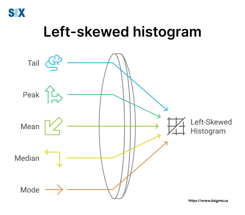
A left-skewed histogram, also known as a negatively skewed histogram, is a graphical representation of data where the tail of the distribution extends towards the left side, with the bulk of the data concentrated on the right.

In simpler terms, when you look at a left-skewed histogram, you’ll notice that the “peak” of the data is shifted towards the right, while there’s a longer tail stretching to the left.

Key characteristics to identify in a left-skewed histogram include:

1. The peak (mode) is on the right side of the center.
2. The tail extends longer on the left side.
3. The mean is typically less than the median.

To help visualize this, imagine you’re looking at a dataset of employee salaries in a company. You might see a large group of employees with higher salaries on the right, and a smaller number of employees with much lower salaries creating that left tail.

Comparing Left Skewed Histogram with Other Distribution Types

To truly understand what a left-skewed histogram looks like, it’s helpful to compare it with other common distribution types I’ve encountered in my consulting work:

1. Normal Distribution: This is the classic “bell curve” shape, symmetrical on both sides. Unlike a left-skewed histogram, the mean, median, and mode are all equal in a normal distribution.
2. Right Skewed Distribution: This is the mirror image of a left-skewed histogram. The tail extends to the right, with the bulk of the data on the left side.
3. Symmetrical Distribution: While similar to a normal distribution, not all symmetrical distributions are normal. The key is that they’re balanced on both sides, unlike our left-skewed histogram.

Understanding these differences is crucial. In my work with companies like Intel and Motorola, I’ve seen how misinterpreting the type of distribution can lead to costly mistakes in process improvement initiatives.

Ready to deepen your understanding of data distributions and their impact on business decisions? Enroll in a short course on statistical analysis and data interpretation.

Properties and Characteristics of a Left Skewed Histogram

Understanding the properties and characteristics of left-skewed histograms is crucial for effective data analysis and decision-making. Let’s dive into these key aspects that I’ve seen make a significant difference in projects across various industries.

Mean, Median, and Mode Relationship

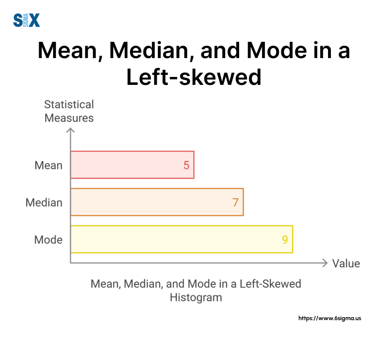
One of the most distinctive features of a left-skewed histogram is the relationship between its mean, median, and mode. In my workshops, I often use this relationship as a quick identifier for left skewness:

Mean < Median < Mode

This relationship is quite different from what we see in normal distributions, where these three measures of central tendency are typically equal. Let me break it down based on my experiences:

1. Mean: In a left-skewed histogram, the mean is pulled towards the left tail by the smaller values. I’ve seen this cause confusion in salary analyses, where the average (mean) salary can be misleadingly low due to a few entry-level positions.
2. Median: The median, being the middle value, is less affected by extreme values. It’s often a more reliable measure of center in skewed distributions.
3. Mode: This is the peak of our distribution, representing the most common value. In left-skewed histograms, it’s the rightmost of these three measures.

Tail and Peak Analysis

Understanding the tail and peak of a left-skewed histogram can provide valuable insights:

1. Long Left Tail: This extended tail represents the less frequent, smaller values in our dataset. In my work with manufacturing processes, I’ve seen this tail represent rare defects or outlier performance issues.
2. Peak Position: The peak (mode) is shifted towards the right side of the distribution. This indicates that the most common values in our dataset are on the higher end of the range.

Skewness Measurement

To quantify the degree of skewness, we use the skewness coefficient:

1. Negative Skewness: A left-skewed histogram will have a negative skewness coefficient. The more negative the value, the more pronounced the left skew.
2. Interpreting Values: In my experience, values between -0.5 and -1 indicate moderate skewness, while values below -1 suggest high skewness. However, these are general guidelines and can vary depending on the specific context of your data.

Key Properties of Left-Skewed Histograms

• The mean is less than the median, which is less than the mode
• The long tail extends to the left
• Peak (mode) is positioned on the right side
• Negative skewness coefficient
• The majority of data points are on the right side
• Fewer, but more extreme, low values on the left

Understanding these properties of left-skewed histograms is essential for accurate data interpretation.

Interpreting a Left Skewed Histogram: A Step-by-Step Guide

In my years of consulting and teaching Six Sigma methodologies, I’ve found that interpreting left-skewed histograms is a crucial skill for data-driven decision-making.

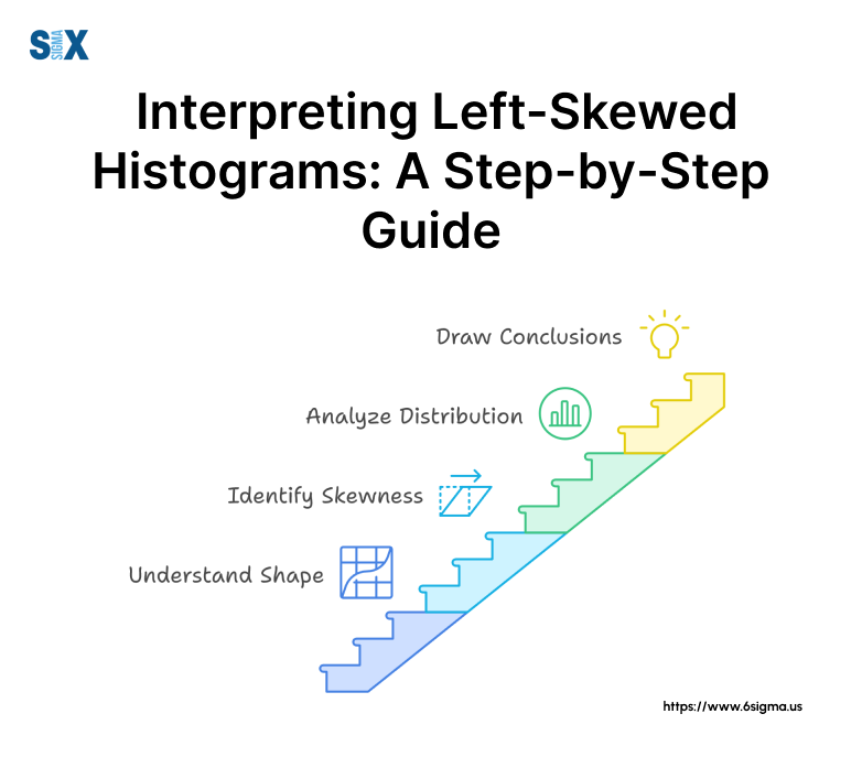
Identifying the Distribution of Shape

The first step in interpreting a left-skewed histogram is recognizing its unique shape. Here’s what to look for:

1. Longer tail on the left side
2. Peak (mode) shifted to the right
3. Gradual slope on the left, steeper slope on the right

Remember, a left-skewed histogram doesn’t always mean there’s a problem. In some cases, it’s the expected distribution. For instance, in a project, we found that the distribution of time-to-failure for certain products was naturally left-skewed.

Analyzing Central Tendency Measures of a Left Skewed Histogram

Understanding the relationship between mean, median, and mode is crucial:

1. Mean < Median < Mode
2. Mean is pulled towards the left tail
3. Median is often more representative of the typical value

In a Six Sigma project, we used this relationship to identify discrepancies in customer satisfaction scores that weren’t apparent from the average alone.

Understanding Data Concentration and Outliers

In a left-skewed histogram:

1. Most data points cluster on the right side
2. Outliers typically appear on the left side
3. The left tail often represents rare but significant events

During a process improvement initiative, we identified critical quality issues by focusing on these left-tail outliers.

Contextualizing the Skewness

Always consider the context of your data:

1. What does the left tail represent in your specific scenario?
2. Is the skewness expected or a sign of an underlying issue?
3. How does the skewness impact your business goals?

Common Pitfalls of a Left Skewed Histogram and How to Avoid Them

Be aware of these common mistakes:

1. Focusing solely on the mean: Always consider median and mode too
2. Ignoring outliers: They often hold valuable insights
3. Assuming normality: Many real-world processes aren’t normally distributed

In a project, we initially missed a crucial insight by falling into the “normality assumption” trap. Always question your assumptions!

Want to apply these interpretation techniques to real-world scenarios? Get hands-on experience with advanced statistical techniques with our Lean Six Sigma Green Belt.

Applications and Examples

These asymmetrical distributions often reveal critical insights that can drive business decisions and process improvements. Let me share some examples from my experience working with global corporations and government institutions.

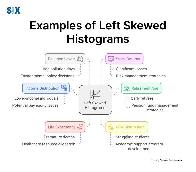
Income Distribution Analysis

One of the most common examples of a left-skewed histogram is income distribution. In a project I led for a large multinational corporation, we analyzed employee salaries across different departments. The resulting left-skewed histogram revealed:

• A large cluster of mid-level salaries on the right
• A long tail to the left represents lower-paid entry-level positions
• A few extremely high salaries pull the mean lower than the median

This analysis helped the company identify potential pay equity issues and informed its compensation strategy.

Age-Related Data

During my work with healthcare organizations, I’ve often encountered left-skewed histograms in age-related data:

1. Retirement Age: A slightly left-skewed histogram typically shows most people retiring around 65, with a tail extending to earlier retirements.
2. Life Expectancy: When analyzing life expectancy data for a government health initiative, we found a left-skewed distribution with a peak around 80 years and a tail extending towards younger ages.

Academic Performance Metrics with a Left Skewed Histogram

In an educational consulting project, we analyzed student performance data:

• GPA distributions often show a left skew, with most students clustered around higher GPAs
• Standardized test scores can also exhibit left skewness, especially for advanced exams

Understanding these distributions helped institutions develop more effective support programs for struggling students.

Environmental Data

Environmental metrics frequently display left skewness:

• Pollution Levels: In a project for an environmental agency, we found that daily air quality readings often produced a left-skewed histogram, with most days having low pollution and a few high-pollution days creating the left tail.
• Rainfall: Analyzing rainfall data for an agricultural client revealed a left-skewed distribution, with most months having moderate rainfall and occasional drought periods forming the left tail.

Financial Markets

Stock returns typically show a left-skewed distribution:

• Most returns cluster around a slightly positive value
• The left tail represents occasional significant losses
• Rare but extreme positive returns create a slight right skew

This distribution underscores the importance of risk management in investment strategies.

These examples demonstrate the ubiquity and importance of left-skewed histograms across various fields. By recognizing and correctly interpreting these distributions, you can uncover valuable insights that drive informed decision-making in your organization.

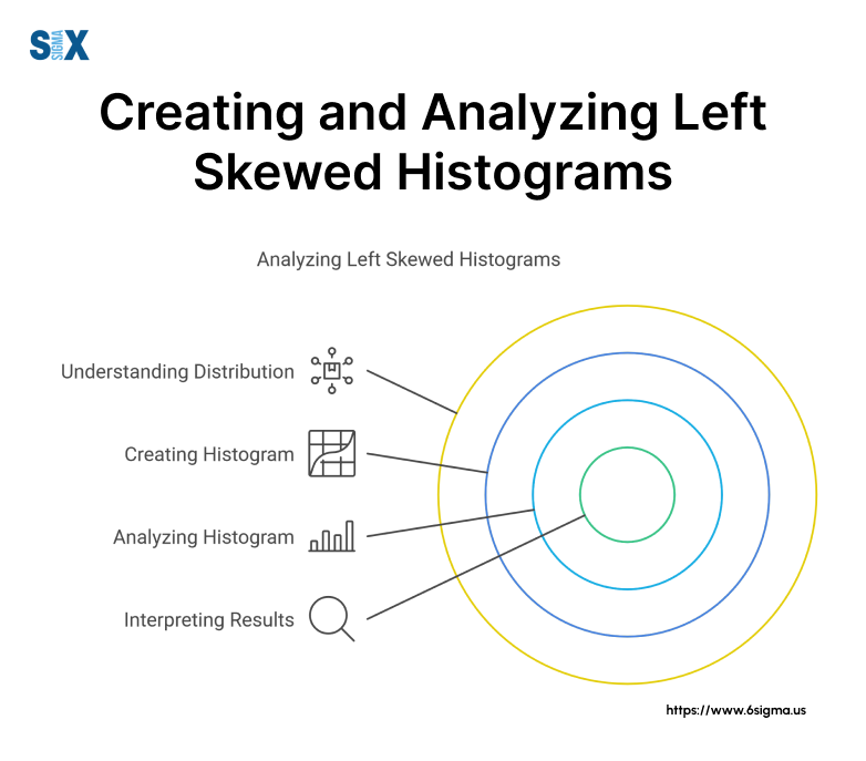
Creating and Analyzing Left Skewed Histograms

Let me share some insights I’ve gained from working with companies and government institutions over the years.

Data Collection Considerations

When dealing with potentially left-skewed data, keep these points in mind:

1. Sample Size: Ensure your sample is large enough to reveal the true distribution. In a project at Motorola, we initially missed a left skew due to insufficient data.
2. Data Quality: Be vigilant about data accuracy. Outliers in left-skewed histograms can be significant, not just errors.
3. Time Frame: For time-series data, consider whether the skewness is consistent or varies over time. This was crucial in a long-term process improvement project.

Choosing Appropriate Bin Sizes for a Left Skewed Histogram

Bin size can significantly impact the appearance of your left-skewed histogram:

1. Too few bins can mask the skewness
2. Too many bins can create noise and obscure the overall pattern
3. Consider using unequal bin widths for highly skewed data

I often use the square root of the sample size as a starting point for the number of bins, adjusting as needed based on the data’s characteristics.

Tools and Software for Histogram Creation

Over the years, I’ve used various tools to create left-skewed histograms:

1. Excel: Great for quick visualizations. Use the Data Analysis ToolPak for basic histograms.
2. R: My go-to for advanced statistical analysis. The ggplot2 package is excellent for customizable histograms.
3. Python Libraries: Matplotlib and Seaborn are powerful for creating histograms, especially when dealing with large datasets.
4. Minitab: A staple in Six Sigma projects, it offers robust histogram capabilities.

Best Practices for Visual Presentation

To effectively communicate your findings:

1. Use clear labeling for axes and bins
2. Include a legend if comparing multiple datasets
3. Consider overlaying a normal distribution curve for comparison
4. Use color strategically to highlight key areas of the distribution

Remember, the goal isn’t just to create a left-skewed histogram, but to use it as a tool for insight and decision-making. In my workshops, I always emphasize that the real value comes from interpreting the histogram in the context of your specific business challenge.

More Topics in Left-Skewed Distributions

These topics are crucial for anyone looking to master data analysis and drive meaningful business improvements.

Transforming Left Skewed Histogram Data

In many Six Sigma projects, I’ve encountered situations where we needed to transform left-skewed data for further analysis:

1. Log Transformation: Often effective for slightly left-skewed histograms, especially in financial data.
2. Box-Cox Transformation: A powerful method I’ve used in manufacturing processes to normalize skewed data.
3. Square Root Transformation: Useful for counting data that shows left skewness.

Remember, the goal of transformation is not just to achieve normality, but to make your data more amenable to statistical analysis while preserving its fundamental characteristics.

Statistical Tests for Skewed Data

When dealing with left-skewed distributions, traditional tests may not be appropriate. Here are some alternatives I frequently use:

1. Mann-Whitney U Test: A non-parametric test I’ve applied in quality control projects.
2. Kruskal-Wallis Test: Useful for comparing multiple groups with skewed data.
3. Bootstrapping Methods: I’ve found these particularly valuable for estimating confidence intervals in skewed datasets.

Implications for Predictive Modeling

Left skewed data can significantly impact predictive models:

1. In regression analysis, skewed residuals can violate assumptions and lead to unreliable predictions.
2. For classification problems, skewed features may need special handling to prevent bias.
3. Time series forecasting with left-skewed data often requires specialized models like GARCH.

During a project, we had to redesign our entire predictive maintenance model due to overlooked left skewness in equipment failure times.

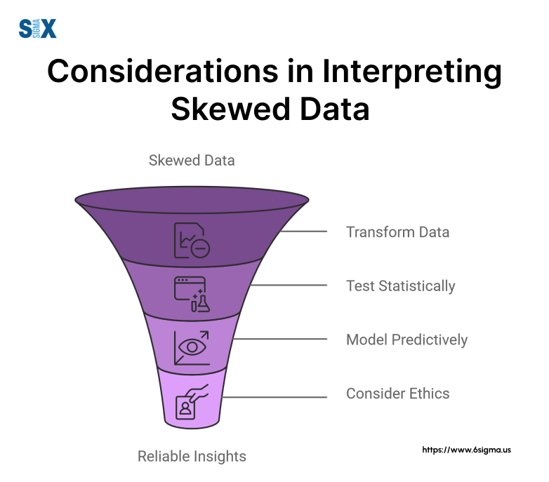
Ethical Considerations in Interpreting Skewed Data

As data scientists and business leaders, we have an ethical responsibility to interpret skewed data correctly:

1. Avoid cherry-picking metrics that hide important information in the left tail.
2. Be transparent about the limitations of your analysis when dealing with skewed distributions.
3. Consider the real-world implications of decisions based on skewed data, especially in sensitive areas like healthcare or finance.

These advanced topics underscore the complexity and importance of understanding left-skewed histograms in real-world scenarios. By mastering these concepts, you’ll be better equipped to extract valuable insights from your data and make informed decisions.

Ready to dive deeper into advanced statistical methods and their applications? Focus on cutting-edge data analysis techniques for process improvement with a short course on Introduction to Graphical Analysis with Minitab.

Historical Context and Future Trends

As a Six Sigma Master Black Belt with over two decades of experience, I’ve witnessed firsthand the evolution of data analysis techniques, particularly in the realm of left-skewed histograms. Let’s take a journey through time and peek into the future of this crucial statistical tool.

Brief History of Skewed Distribution Analysis

The concept of skewed distributions dates back to the late 19th century, but its practical applications have grown exponentially:

1. 1895: Karl Pearson introduced the concept of skewness in distributions.
2. 1920s: R. Fisher developed methods for handling non-normal distributions.
3. 1960s: Box-Cox transformations emerged, revolutionizing how we handle skewed data.
4. 1980s: Robust statistical methods gained popularity, addressing challenges with skewed data.

During the 1990s, I saw a shift from avoiding skewed data to embracing it for deeper insights.

Emerging Applications in Big Data and Machine Learning

The big data revolution has brought new relevance to left-skewed histograms:

1. Anomaly Detection: In cybersecurity projects I’ve led, left-skewed distributions often indicate potential threats.
2. Predictive Maintenance: At companies like GE, we’ve used skewed time-to-failure distributions to optimize maintenance schedules.
3. Customer Behavior Analysis: E-commerce giants are leveraging skewed purchase patterns for personalized marketing.

Machine learning algorithms are becoming more adept at handling skewed data, opening up new possibilities for automated analysis and decision-making.

Predicted Developments of a Left Skewed Histogram in Data Visualization Techniques

The future of left-skewed histogram analysis is exciting:

1. Interactive 3D Visualizations: I’m seeing prototypes that allow users to “walk through” skewed distributions in virtual reality.
2. Real-time Dynamic Histograms: Imagine dashboards that update left-skewed histograms as data streams, something we’re implementing in IoT projects.
3. AI-assisted Interpretation: Tools that not only display left-skewed histograms but provide context-aware insights are on the horizon.

As we move forward, the ability to understand and leverage left-skewed histograms will become increasingly crucial. I can confidently say that mastering these concepts will be a key differentiator in data-driven decision-making.

Going Forward

As we wrap up our deep dive into left-skewed histograms, I want to emphasize the critical role these statistical tools play in modern business and project management. I’ve seen firsthand how understanding left-skewed distributions can lead to breakthrough insights and drive meaningful improvements.

Let’s recap the key points we’ve covered:

1. We defined what a left-skewed histogram is and explored its unique characteristics.
2. We examined the crucial relationship between mean, median, and mode in left-skewed distributions.
3. We discussed real-world applications across various industries, from finance to manufacturing.
4. We delved into advanced topics like data transformation and ethical considerations.
5. Finally, we looked at the historical context and future trends in skewed data analysis.

Understanding left-skewed histograms is not just about statistical knowledge – it’s about gaining a deeper understanding of your processes, customers, and business environment.

If you’re ready to take your data analysis skills to the next level, consider exploring our advanced Six Sigma courses at SixSigma.us. Together, we can turn your data into actionable insights that drive real business results.