Degrees of Freedom in Statistics. Everything You Need to Know

Degrees of opportunity (df statistics) assume a fundamental part in deciding investigation exactness and legitimacy.

Regardless of whether directed speculation tests, fitting relapse models, or exploring information, understanding df statistics is pivotal for drawing educated ends.

Degrees of flexibility speak to the measure of figures free to fluctuate amid factual computations.

It measures how much the information may give for anticipating parameters or testing suspicions. Higher df implies more information focus adding to examination, accomplishing all the more dependable and exact gauges.

Key Highlights

• Degrees of flexibility (df statistics) speak to the significance measured to information concentrates on factual estimations.
• Understanding df is basic for rightfully deciphering outcomes from exploration, relapse examination, and models.
• Df statistics relies upon example estimates and parameters decided from the information. More df proposes more dependable outcomes; bringing down df lessens trust in discoveries.
• Reporting df alongside factual insights permits a fitting assessment of centrality and impacts.
• Df estimations contrast somewhat over t-tests, ANOVA, chi-square, and different tests. Statistic programs like R, Python, and SPSS assistance acquire df yields amid examinations.

What is Degrees of Freedom (df) in Statistics?

In measurements, degrees of opportunity (df) in statistics play a fundamental part in various investigations and suspicion testing techniques.

Df statistics speaks to freely changing estimations. Understanding df is fundamental for deciphering factual tests, anticipating parameters, and drawing sound deductions from information.

Df connects to example estimates and parameters chosen. It measures readily available data for making suppositions or testing suspicions. More df proposes more exactness.

Df rose from limitations on focuses or observations. For this case, a solitary esteem relies upon others, diminishing flexible regards by one. This mirrors df decreases.

Df statistics assumes pivotal jobs in t-tests, ANOVA, chi-square, and F-tests, deciding correct disseminations and basic qualities. Additionally, df helps assess model precision.

Degrees of Freedom (df) Statistics in Hypothesis Testing

Degrees of freedom (df) in statistics play a crucial role in hypothesis testing, which is a fundamental concept in statistical inference.

Hypothesis tests are used to determine whether the results from sample data are statistically significant and can be generalized to the larger population. The degrees of freedom help determine the appropriate distribution to use when calculating test statistics and p-values.

In hypothesis testing, there are generally two main types of tests:

1. Tests about a population mean (e.g. one-sample t-test, two-sample t-test)
2. Tests about population proportions or variances (e.g. chi-square, F-test, ANOVA)

The degrees of freedom vary depending on the specific test being conducted.

For tests about a population mean using the t-distribution:

• One-sample t-test: df = n – 1 (where n is the sample size)
• Two-sample t-test: df = n1 + n2 – 2 (where n1 and n2 are the sample sizes)

For tests about proportions using the chi-square distribution:

• Chi-square test for goodness of fit: df = k – 1 (where k is the number of categories)
• Chi-square test for independence: df = (r-1)(c-1) (where r and c are the numbers of rows and columns)

For tests about variances using the F-distribution (e.g. ANOVA, regression):

• The df has two values, one for the numerator and one for the denominator based on sample sizes

Having the correct degrees of freedom is essential for finding the critical values to determine if the test statistic is statistically significant for a given alpha level. Misspecifying the df can lead to invalid statistical conclusions.

Calculating Degrees of Freedom (dF) Statistics

The calculation of degrees of freedom depends on the specific statistical test being used. However, some general principles apply across many of the common tests.

For a single sample:

df = n – 1

Where n is the sample size.

For example, if you have a sample of 25 observations, the degrees of freedom would be 25 – 1 = 24.

For two samples:

df = n1 + n2 – 2  

Where n1 and n2 are the sample sizes.

So if you had two independent samples with 18 and 22 observations respectively, the degrees of freedom would be 18 + 22 – 2 = 38.

In the analysis of variance (ANOVA), the degrees of freedom have both a numerator and denominator component related to the sources of variation being estimated. The total degrees of freedom is one less than the total sample size.

For linear regression models, the degree of freedom for error is the sample size minus the number of parameters estimated in the model, including the intercept.

No matter the statistical test, the degrees of freedom represent the data points available to estimate the underlying parameters or sources of variation. Calculating the proper degrees of freedom is crucial for obtaining accurate p-values, confidence intervals, and making appropriate statistical inferences from your data analysis.

Interpretation of Degrees of Freedom (df) in Statistics

The degree of freedom (df) in statistics is an important concept to understand when conducting statistical tests and analyzing data. It represents the number of values in a statistical analysis that are free to vary after certain restrictions or constraints have been imposed. The interpretation of df depends on the specific statistical test or model being used.

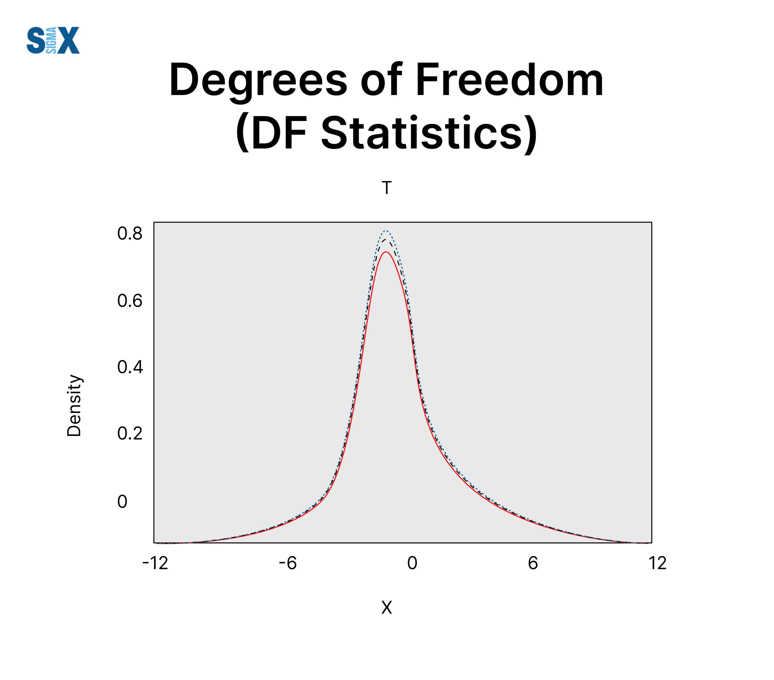
In hypothesis testing, the df statistics helps determine the shape of the probability distribution used to calculate the p-value for assessing statistical significance. A lower df leads to a distribution with thicker tails, making it harder to achieve statistical significance. Conversely, a higher df results in a distribution more closely approximating the normal distribution.

For example, in a one-sample t-test, the df is equal to n-1, where n is the sample size. The df impacts the spread of the t-distribution and the critical t-value needed to reject the null hypothesis. With a small df (e.g. 5), the tails are thicker, so a larger t-statistic is required compared to a scenario with a larger df (e.g. 30).

In ANOVA models, the df represents the divisor used to calculate the mean square values for the between-groups variance (df = k-1 for k groups) and the within-groups variance (df = N-k for N total observations). These df values are used in the F-test statistic.

For chi-square tests, the df indicates which chi-square distribution to use and is equal to (r-1)(c-1) for a contingency table with r rows and c columns. The df impacts the critical chi-square value needed for significance.

In linear regression, the df for the overall model is n-p-1, where n is the sample size and p is the number of predictors. The df for each regression coefficient is the model’s residual df. More predictors decrease the residual df.

The df statistics is crucial for determining the appropriate reference distribution, critical values, and statistical significance for a wide range of analyses.

Degrees of Freedom in Regression and Other Models

Degrees of freedom play a crucial role in regression analysis and other statistical modeling techniques. In regression, the degrees of freedom refer to the number of values that are free to vary after estimating the model parameters.

Linear Regression

In a simple linear regression model with one predictor variable, the degrees of freedom is calculated as n – 2, where n is the total number of observations.

The 2 represents the two parameters estimated in the model – the slope and the intercept. For multiple linear regression with k predictor variables, the degrees of freedom is n – (k + 1).

Having sufficient degrees of freedom is important for obtaining reliable estimates and inferences from the regression model. More degrees of freedom leads to more precise estimates of the regression coefficients and narrower confidence intervals.

Analysis of Variance (ANOVA)

ANOVA models are used to compare means across more than two groups. The degrees of freedom in ANOVA is divided into two components – degrees of freedom for the model and degrees of freedom for error. 

The model degrees of freedom represent the number of parameters estimated, excluding the overall mean. For a one-way ANOVA with k groups, the model df is k – 1. The error degrees of freedom is the remaining degrees of freedom after accounting for the model, calculated as n – k.

Having more error degrees of freedom increases the power and reliability of the F-test used in ANOVA for detecting differences between group means.

Generalized Linear Models within DF Statistics

Generalized linear models extend regression to non-normal response distributions like binary, count, or gamma. The degrees of freedom calculation depends on the specific GLM being fit. For example, in logistic regression for binary data, the model df is the number of predictor variables.

Bayesian Models

In Bayesian analysis, the concept of degrees of freedom is less emphasized compared to frequentist methods. However, it can play a role in specifying priors and evaluating model complexity.

Reporting and Communicating Degrees of Freedom

Properly reporting and communicating the degrees of freedom is crucial when presenting statistical analysis results. The degrees of freedom provide important context about the precision and reliability of your findings.

When reporting test statistics like t, F, or chi-square values, the associated degrees of freedom must also be reported. For example, you might report “t(23) = 2.41, p = 0.024” for a one-sample t-test. The degrees of freedom value of 23 indicates this was based on a sample of 24 observations.

For regression models, report the degrees of freedom for the overall model fit as well as the degrees of freedom for each predictor’s test. For example: “F(3, 42) = 5.87, p = 0.002, R2 = 0.30” shows the model had 3 predictors and 42 residual degrees of freedom.

Communicate what the degrees of freedom represent – whether it is residual/error df, df for the numerator, df for the denominator, etc. This clarifies whether a larger or smaller df corresponds to higher precision.

When interpreting p-values, note that with larger degrees of freedom, smaller p-values are required for significance at a given alpha level. So a p = 0.049 may be significant with df = 20 but not with df = 120.

Data visualizations like error bars on means can also depict the degrees of freedom variation. Smaller sample sizes will have wider confidence interval bars.

Ultimately, reporting degrees of freedom allows others to understand the precision and generalizability of your statistical results. It provides crucial context, so be diligent about calculating, reporting, and interpreting them properly.

Conclusion and Additional Resources

In conclusion, understanding degrees of freedom (df) in statistics is crucial for properly interpreting statistical tests and making valid inferences from data.

The df represents the number of values that are free to vary after certain restrictions or constraints have been imposed by the statistical model or hypothesis test.

The df statistics plays a key role in hypothesis testing by determining the shape of the probability distribution used for calculating p-values and critical values. It also influences the precision of parameter estimates and the width of confidence intervals in methods like linear regression.