Articles

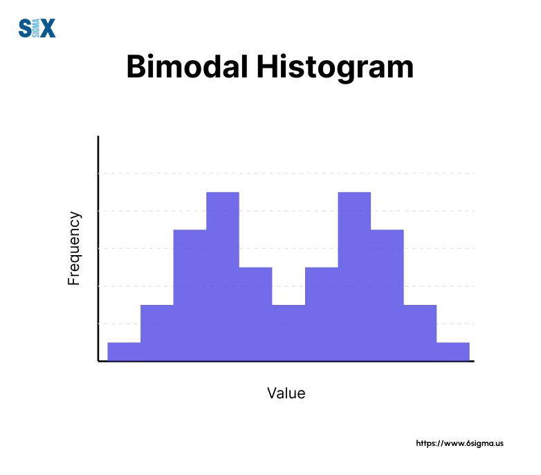
A bimodal histogram graphically depicts data exhibiting two distinct peaks in the distribution or modes.

This signifies two separate groups or processes within a single dataset.

Various factors can produce such a unique pattern, like merged operations, combined populations, or natural bimodality seen in some study fields.

Key Highlights

• Understand bimodal distributions and their graphical representation
• Explore the common causes of bimodal distributions
• Identify bimodal histogram shapes and distinguish them from unimodal distributions
• Discover practical applications of the bimodal histogram
• Step-by-step process of creating and interpreting bimodal histograms
• Gain insights into analyzing bimodal data
• Explore examples and case studies
• Future directions and emerging trends in bimodal analysis

Understanding Bimodal Distributions and Their Histograms

In data analysis, it is crucial to grasp the concept of bimodal distributions and their visual representation through bimodal histograms.

A bimodal distribution is a type of probability distribution that exhibits two distinct peaks or modes, indicating the presence of two separate groups or processes within the same dataset.

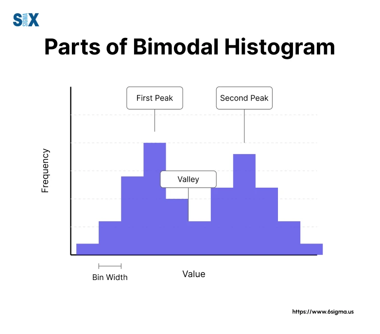
The key characteristic of a bimodal distribution is the existence of dual peaks, which reflect the concentration of data points around two different values or ranges.

These peaks are separated by a visible valley or trough, creating a distinctive “double-humped” shape on the histogram.

The modes of a bimodal distribution represent the most frequently occurring values or ranges in the data.

Each mode corresponds to a local maximum, indicating a high density of observations clustered around that particular value or range.

Identifying and analyzing these modes is crucial for understanding the underlying dynamics and potential subpopulations within the data.

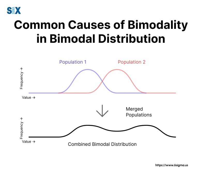
What Causes Bimodal Distributions?

Bimodal distributions can arise from various sources, and understanding these causes is essential for interpreting the data accurately.

Here are some common scenarios that can lead to bimodal patterns:

1. Merged processes: When two processes or mechanisms are combined or merged, the resulting dataset may exhibit a bimodal distribution. Each process contributes to one of the modes, reflecting its unique characteristics or outcomes.
2. Combined populations: In certain cases, data may be collected from two populations or subgroups with distinct characteristics or behaviors. When these subpopulations are combined into a single dataset, a bimodal distribution can emerge, with each mode representing one of the subpopulations.
3. Natural bimodal phenomena: Some phenomena in nature or specific fields of study inherently exhibit bimodal patterns. For example, the size distribution of Weaver ants and the age of onset for Hodgkin’s Lymphoma are known to follow bimodal distributions due to their underlying biological or disease mechanisms.

Bimodal distribution examples:

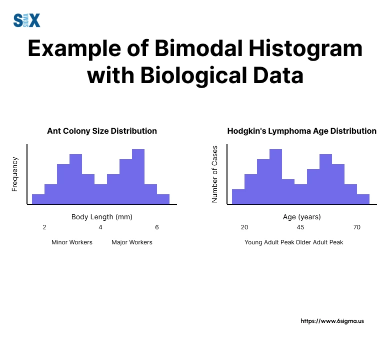
• Weaver ants: The body lengths of worker ants within a colony exhibit a bimodal distribution, with smaller ants acting as caretakers and larger ants responsible for nest construction and defense.
• Hodgkin’s Lymphoma: The age of onset for this type of cancer follows a bimodal pattern, with peaks occurring in young adulthood and again in older age groups.

Identifying Bimodal Histogram

Recognizing bimodal histograms is crucial for detecting the presence of bimodal distributions within a dataset.

A bimodal histogram is characterized by its distinctive shape, which features two humps or peaks separated by a visible trough or valley.

The histogram shape of a bimodal distribution is often described as “symmetric bimodal” when the two peaks are roughly equal in height and separated by a central valley.

However, it is also possible to encounter asymmetric bimodal histograms, where one peak is higher or more pronounced than the other.

To identify a bimodal histogram, it is essential to inspect the graphical representation of the data distribution visually.

The presence of two humps or modes, separated by a noticeable gap or trough, is a clear indicator of a bimodal pattern.

Practical Applications of Bimodal Histogram

Bimodal histograms and the analysis of bimodal distributions have practical applications across various fields and industries.

Here are some examples:

1. Genetics (gene expression analysis): Bimodal histograms can be used to identify gene expression levels and two active groups in different conditions, helping uncover new disease pathways or drug targets.
2. Marketing (customer satisfaction analysis): By analyzing customer satisfaction levels through bimodal histograms, businesses can identify two different customer groups with different satisfaction levels, allowing for targeted marketing and customer service strategies.
3. Finance (stock market analysis): Bimodal histograms can provide insights into stock price behavior and other financial indicators, assisting investors in making informed decisions based on market trends and patterns.
4. Manufacturing (product defect analysis): By analyzing product defects using bimodal histograms, manufacturers can identify two defect groups, potentially caused by different factors, and implement targeted quality control measures.
5. Education (test score analysis): Bimodal histograms can help educators identify groups of students with different performance levels, enabling them to provide appropriate support or enrichment programs.
6. Psychology (personality analysis): In the field of psychology, bimodal histograms can be used to analyze personality traits and identify distinct groups with different characteristics, aiding in the development of personalized treatments or interventions.

Creating and Interpreting Bimodal Histogram

It is essential to follow a systematic approach to create and interpret bimodal histograms effectively.

Here are the key steps involved:

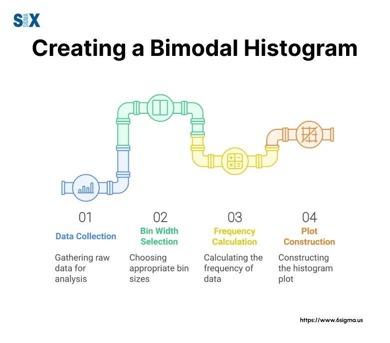
1. Data collection: Gather the relevant data for which you want to create a bimodal histogram. Ensure that the data is numerical and continuous.
2. Bin width selection: Choose an appropriate bin width, which determines the size of the bars on the histogram. A smaller bin width will provide more detail, but it may also result in a cluttered or noisy histogram.
3. Frequency calculation: Divide the data range into bins of equal width and count the number of observations falling within each bin. This will give you the frequency or number of data points per bin.
4. Histogram construction: Plot the bins on the x-axis and their corresponding frequencies on the y-axis. Drawbars of equal height above each bin to create the histogram.
5. Mode identification: Visually inspect the histogram and identify the two peaks in the distribution or modes, which represent the most frequently occurring values or ranges in the data.
6. Axis labeling: Clearly label the x-axis with the variable being measured and the y-axis with the frequency or relative frequency.
7. Result analysis: Analyze the bimodal histogram to identify trends, patterns, or anomalies. Interpret the position and height of the peaks and the valley between them to gain insights into the underlying data and potential subpopulations or processes.

Distinguishing Bimodal Histogram from Unimodal Distributions

To fully understand bimodal distributions, it is essential to distinguish them from unimodal distributions, which have only one peak or mode.

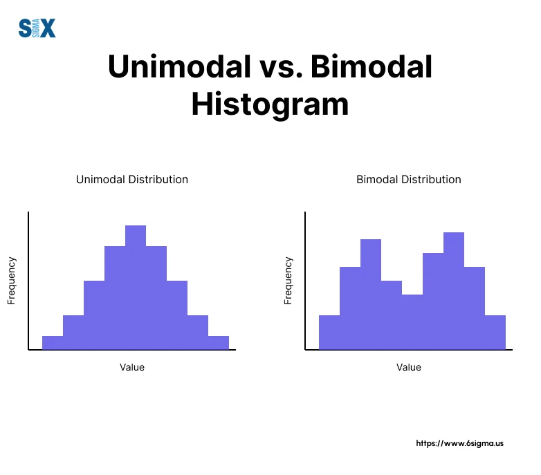
Unimodal distribution: It’s a probability distribution that has a single peak or mode, representing the most frequently occurring value or range in the data.

Bimodal distribution: A bimodal distribution, on the other hand, defines two peaks or modes, indicating the presence of two separate groups or processes within the same dataset.

Shape comparison: The shape of this distribution typically resembles a symmetric bell curve or a skewed distribution with a single high point. In contrast, a bimodal distribution has a distinct “double-humped” shape, with two visible peaks separated by a valley or trough.

Modality differences: The key difference between unimodal and bimodal distributions lies in their modality, which refers to the number of modes or peaks present in the distribution.

Unimodal distributions have a single mode, while bimodal or multimodal distributions have two modes.

Analyzing Bimodal or Multimodal Data

Analyzing bimodal data requires a careful approach to ensure accurate interpretation and reliable statistical analysis.

Here are some key considerations:

1. Separating subpopulations: If the bimodal distribution arises from the combination of two subpopulations or processes, separating the data into these subgroups is often beneficial for further analysis. This allows for a more detailed examination of each subpopulation’s characteristics and patterns.
2. Central tendency measures (mean, median): In bimodal distributions, the mean and median may not accurately represent the central tendency of the data, as they can fall between the two modes, where fewer observations exist. It is essential to interpret these measures cautiously and consider alternative measures, such as the mode itself or separate measures for each subpopulation.
3. Variability measures (standard deviation, range): Bimodal distributions can exhibit larger variability when analyzed as a single dataset. Separating the data into subpopulations can provide more precise measures of variability, such as the standard deviation or range, for each group.
4. Reliable statistical analysis: Failing to account for the bimodal nature of the data can lead to unreliable statistical analyses and erroneous conclusions. It is crucial to recognize the presence of bimodal patterns and adjust the analytical approaches accordingly, such as by separating subpopulations or employing specialized statistical techniques.

Challenges and Pitfalls of Bimodal Histogram

While bimodal distributions can provide valuable insights, they also present several challenges and potential pitfalls that must be addressed:

1. Misinterpreting combined data: Analyzing combined data without recognizing the underlying bimodal pattern can lead to misleading conclusions and inaccurate interpretations. It is essential to identify and separate the subpopulations or processes contributing to the bimodal distribution.
2. Overlooking underlying causes: Failing to investigate the potential causes or mechanisms behind the bimodal distribution can result in a superficial understanding of the data. It is crucial to explore the underlying factors that contribute to the formation of distinct subpopulations or processes.
3. Incorrect conclusions: Drawing conclusions based solely on traditional statistical summaries, such as the mean or median, without considering the bimodal nature of the data can lead to incorrect inferences and flawed decision-making.
4. Unreliable statistical summaries: Statistical summaries, such as measures of central tendency and variability, may not accurately represent the characteristics of bimodal data when treated as a single distribution. It is essential to interpret these summaries with caution and consider alternative measures or techniques tailored to bimodal patterns.

Examples and case studies

To further illustrate the importance and applicability of bimodal histogram analysis, let’s explore some examples.

Industry-specific examples

• Manufacturing: In a Six Sigma project at a leading automotive company, we encountered a bimodal distribution in the surface finish of a critical component. Upon investigation, we discovered that two different machining processes were being used, resulting in distinct quality outcomes. By separating the data and optimizing each process individually, we significantly improved product quality and consistency.
• Finance: During a risk assessment project for a major financial institution, we analyzed the credit scores of their customer base. The bimodal histogram revealed two different customer segments with different risk profiles. This insight enabled the institution to develop targeted risk management strategies and tailor their services accordingly.

Research case studies

• Ecology: In a study on the population dynamics of a particular bird species, researchers observed a bimodal distribution in the wing length measurements. This pattern was attributed to the presence of two distinct subpopulations, possibly due to geographic isolation or genetic factors. Further investigations provided valuable insights into the species’ evolution and conservation efforts.
• Psychology: A bimodal distribution was observed in a study analyzing the response times of participants during a cognitive task. The two modes were hypothesized to represent different cognitive strategies employed by the participants. This finding led to a deeper understanding of the underlying cognitive processes and potential individual differences.

Data visualization techniques

• Interactive visualizations: Leveraging interactive data visualization tools, we can create dynamic bimodal histogram representations that allow users to explore the data, adjust bin widths, and investigate potential subpopulations or processes contributing to the bimodal pattern.
• Overlay analysis: By overlaying bimodal histograms from different datasets or periods, we can identify shifts or changes in the distribution patterns, providing insights into evolving trends or emerging subpopulations.

Insights and findings

• Through the analysis of bimodal histograms, we have gained valuable insights into various phenomena, such as product quality variations, customer segmentation, ecological dynamics, and cognitive processes.
• These insights have enabled data-driven decision-making, process optimizations, targeted interventions, and a deeper understanding of the underlying mechanisms driving the observed bimodal patterns.

Bimodal Distribution in Lean Six Sigma

Central to Lean Six Sigma is data-driven decision-making, aiming to enhance quality, reduce variation, and eliminate waste. Bimodal distributions can signify complex process behaviors, requiring a thoughtful approach to process improvement:

• Identifying Process Variance: Understanding bimodal distributions allows you to uncover underlying issues in processes, particularly when two distinct processes are merged, leading to ineffective problem-solving if interpreted as a single process.
• Root Cause Analysis: In the ‘Analyze’ phase of DMAIC, recognizing bimodal distributions may point out segments of the process requiring specific investigations or separate improvement strategies.

Applications in DMAIC or DMADV Methodologies

Bimodal distribution can be utilized across various stages of DMAIC (Define, Measure, Analyze, Improve, Control) or DMADV (Define, Measure, Analyze, Design, Verify):

• Define: When defining the problem or project scope, acknowledging bimodal patterns can clarify objectives by identifying distinct populations or processes that may need different approaches.
• Measure: In this phase, measurements can include constructing bimodal histograms to visualize process variations and share insights with the team, illuminating the presence of separate groups.
• Analyze: Bimodal distributions are especially valuable in this phase. Practitioners can separate the data into subgroups to understand differing behaviors, potentially leading to distinct root causes for each mode. For example, in a manufacturing context, two peaks in defect rates could correspond to different production lines with distinct issues.
• Improve: The analysis of bimodal data can promote targeted interventions for each subgroup. For instance, if customer satisfaction reveals two distinct patterns, businesses can implement personalized strategies tailored to each group.
• Control: In the Control phase, continuous monitoring of bimodal distributions can alert teams to shifts in process performance, ensuring the appropriate measures remain in place.

How Bimodal Distribution Fit into the Lean Six Sigma Framework

The bimodal analysis complements Lean Six Sigma tools such as:

• Value Stream Mapping: Identifying where waste occurs in each mode can improve efficiency.
• Root Cause Analysis (RCA): Recognizing distinct causes for variation in processes highlighted by bimodal distributions can lead to a more effective RCA.
• Control Charts: Integrating bimodal insights into control charts can provide a clearer picture of process stability over time.

Benefits for Six Sigma Practitioners

Understanding bimodal distributions enhances decision-making capabilities across different levels:

• Green Belts can effectively utilize bimodal analysis to assist in scope definition and data collection processes.
• Black Belts can leverage bimodal insights during root cause analysis, facilitating distinction between different process flows.
• Master Black Belts can use bimodal data to drive company-wide improvements and training programs, ensuring overall alignment in data analysis techniques across projects.

The Role of Bimodal Distribution in Process Improvement Goals

Bimodal distributions play a critical role in Lean Six Sigma goals:

• Reducing Variation: Identifying bimodal patterns helps practitioners focus on the sources of variation, leading to better-specific interventions that address the unique characteristics of each subgroup.
• Eliminating Waste: Understanding the distinct processes contributing to a bimodal dataset allows the elimination of unnecessary steps, thereby streamlining operations.
• Enhancing Quality: By understanding the dualities in data distributions, you can improve quality by addressing the specific needs of varied customer segments or product lines that otherwise get overlooked in a single-mode analysis.

Future Directions and Emerging Trends

As data assumes growing importance across fields, bimodal distribution and histogram examination will remain pivotal.

Advanced analysis methods will likely emerge.

Specialized statistical techniques and algorithms promise more precise modeling and insights. Machine learning and AI integration may automate the detection and characterization of large datasets.

Machine learning shows potential in isolating bimodal subsets or processes within intricate compilations. Predictions accounting for bimodality could enhance forecasting and decisions.

Handling and comprehending bimodality within big data scales presents opportunities. Integration into large-scale analytics pipelines and live oversight systems envisions improving with technological evolution.

Overall, elucidating bimodality’s nuances equips drawing inferences from complete vantage points. Its role in evidence-led resolutions will likely amplify amid the data’s permeating significance.

Advancements may uncover previously obscure intricacies, so diligently tracking innovations merits consideration.

Maintaining proficiency helps maximize bimodality’s problem-solving gifts, wherever applicable.

Frequently Asked Questions About Bimodal Histogram