Articles

Similar characteristics are determined in multiple groups of data which requires statistical analysis.

To assess different groups which have equal variances, Bartlett’s test is the tool you need!

Key Highlights

• Mathematical foundations of the test
• Steps for test implementation
• Result interpretation guidelines
• Applications across various fields
• Software tools for analysis

What is Bartlett’s Test?

A property known as homogeneity of variances is examined by Bartlett’s test whether multiple groups in a dataset have equal variances.

This statistical procedure proves essential when researchers need to validate assumptions before conducting more advanced analyses, such as ANOVA or regression models.

Purpose and Applications of Bartlett’s Test

The primary function of Bartlett’s test for equal variances is to verify that different groups within a dataset exhibit similar levels of variability.

This verification becomes crucial in research scenarios where multiple treatment groups require comparison.

For instance, when studying the effects of different medications on blood pressure, researchers must first confirm that the variance in measurements remains consistent across all treatment groups.

Null and Alternative Hypotheses

The test operates under specific hypotheses:

Null Hypothesis (H0): All group variances are equal
Alternative Hypothesis (Ha): At least one group has a different variance

When the test produces a p-value below the chosen significance level (typically 0.05), researchers reject the null hypothesis, indicating unequal variances among groups.

Bartlett’s Test Assumptions and Limitations

Bartlett’s test relies on several key assumptions:

The data within each group follows a normal distribution. This requirement makes the test particularly sensitive to departures from normality.

When data shows signs of non-normal distribution, statisticians often recommend alternative methods like Levene’s test.

The observations within each group must be independent. This means one measurement should not influence another measurement within the same group.

The test shows particular sensitivity to outliers and extreme values, which can significantly impact results. Therefore, researchers should carefully examine their data for unusual observations before applying the test.

This statistical tool maintains widespread use in quality control, scientific research, and data analysis across various fields.

However, practitioners should consider its limitations and assumptions when deciding whether Bartlett’s test suits their specific analytical needs.

The Mathematics Behind Bartlett’s Test

The statistical foundation of Bartlett’s test involves specific mathematical components that work together to assess variance homogeneity across groups.

The calculation process follows a structured approach using sample data to compute the test statistic.

Bartlett’s Test Statistic Formula

The Bartlett test statistic (B) is calculated using the following formula:

B = [(N-k) ln(s²p) – Σ(ni-1)ln(s²i)] / C

Where:
N = total sample size
k = number of groups
s²p = pooled variance
s²i = variance of the ith group
ni = sample size of the ith group
C = correction factor

The correction factor C adjusts for small sample sizes and is calculated as:
C = 1 + [1/3(k-1)][Σ(1/ni-1) – 1/(N-k)]

Degrees of Freedom

The test operates with k-1 degrees of freedom, where k represents the number of groups being compared.

This value determines the critical region for the test statistic and influences the decision-making process when interpreting results.

Critical Values and P-Value Interpretation

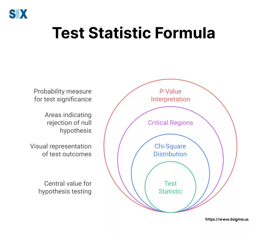
The test statistic follows a chi-square distribution. When analyzing results:

A larger test statistic indicates greater evidence against the null hypothesis of equal variances.

The calculated p-value represents the probability of observing such extreme results under the null hypothesis. Statistical software typically provides these values automatically.

For example, if testing three groups with a significance level of 0.05:

• Test statistic = 7.82
• Degrees of freedom = 2
• P-value = 0.02

This result would indicate significant evidence against equal variances, as the p-value falls below the conventional 0.05 threshold.

Step-by-Step Guide to Performing Bartlett’s Test

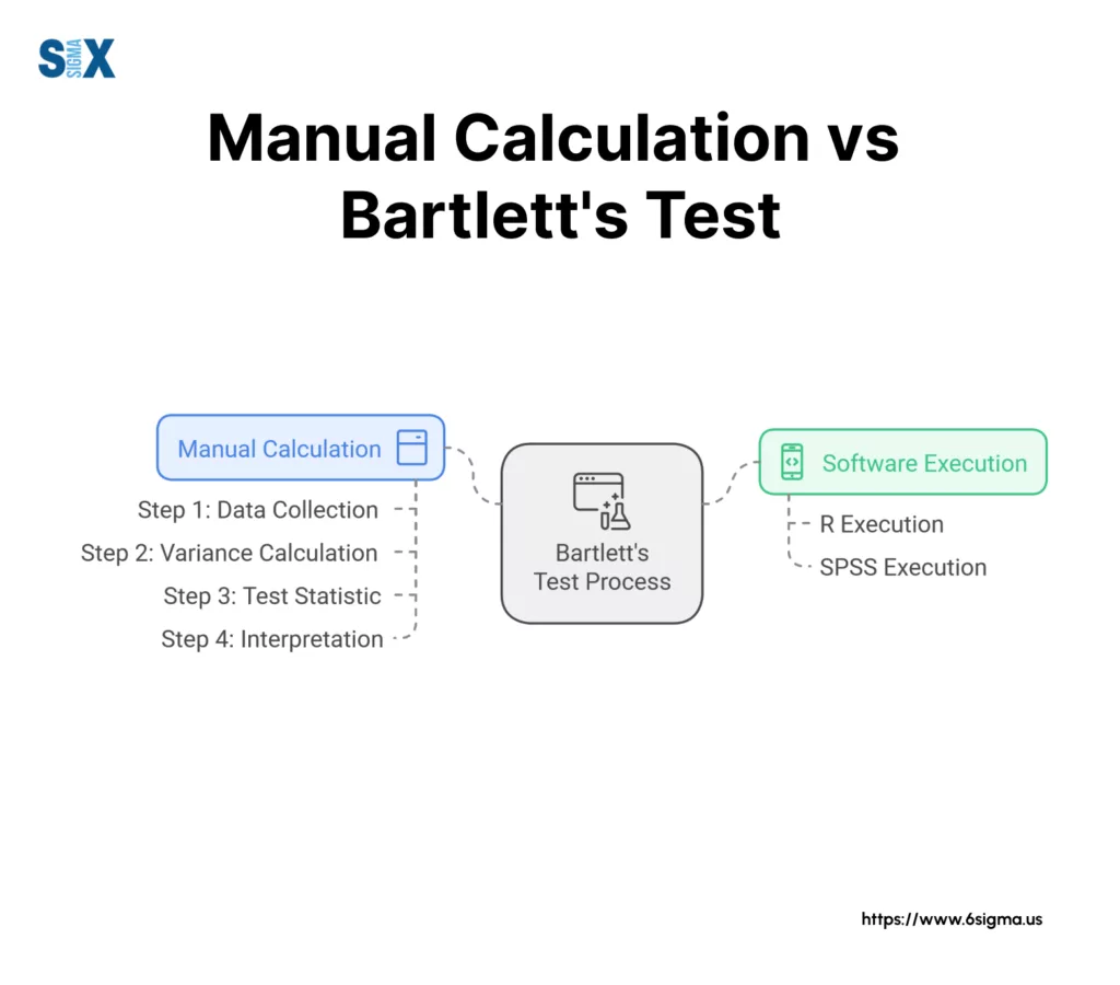
The execution of Bartlett’s test can be approached through manual calculations or statistical software.

Both methods yield identical results when performed correctly, though software solutions offer greater efficiency for large datasets.

Manual Calculation Process

The manual calculation of Bartlett’s test follows these sequential steps:

1. Calculate the variance for each group in the dataset
2. Determine the sample size of each group
3. Compute the pooled variance using all groups
4. Calculate the correction factor (C)
5. Apply the test statistic formula
6. Compare the result with critical values from chi-square distribution

For example, given three groups of data with sample sizes n1=5, n2=5, and n3=5, first calculate individual variances, then proceed with the pooled variance calculation.

The process requires careful attention to maintain mathematical accuracy throughout each step.

Using Statistical Software for Bartlett’s Test

Modern statistical packages simplify the execution of Bartlett’s test through built-in functions:

R Statistical Software:

bartlett.test(variable ~ group, data = dataset)

SPSS:
Navigate to Analyze > Compare Means > One-Way ANOVA > Options > Homogeneity of Variance Test

Excel:
While Excel lacks a direct function for Bartlett’s test, users can create custom formulas or utilize add-in packages designed for statistical analysis.

Output Interpretation

Statistical software typically generates:

• Test statistic value
• Degrees of freedom
• P-value
• Warning messages for potential assumption violations

These outputs require careful interpretation within the context of the research question and chosen significance level.

The choice between manual calculation and software implementation often depends on dataset size, time constraints, and the need for detailed documentation of the analysis process.

Interpreting Bartlett’s Test Results

The interpretation of Bartlett’s test results requires careful consideration of both the p-value and the context of the research question.

Statistical significance in this test carries specific implications for subsequent analyses.

Understanding The P-Value

The p-value from Bartlett’s test indicates the probability of observing the calculated test statistic, assuming equal variances across groups.

A smaller p-value suggests stronger evidence against the assumption of equal variances.

When analyzing the p-value:
P-value < 0.05 indicates significant evidence against equal variances
P-value ≥ 0.05 suggests insufficient evidence to reject the assumption of equal variances

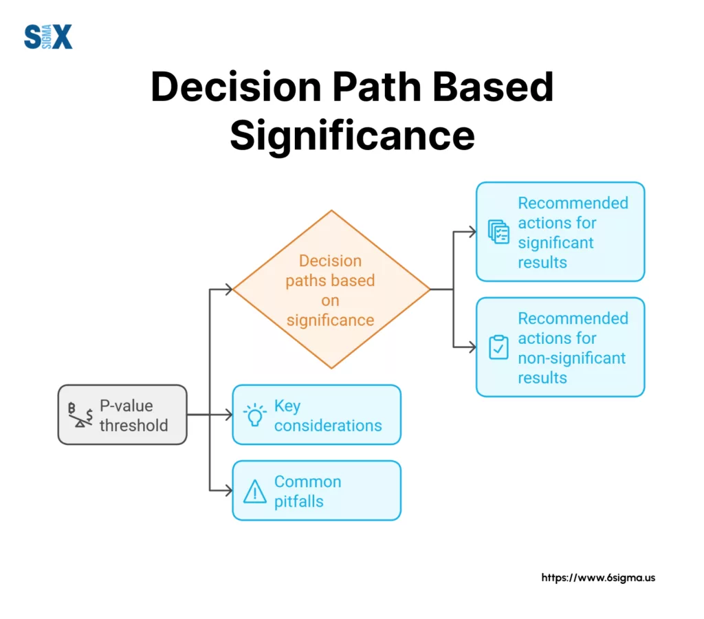
Making Statistical Decisions with Bartlett’s Test

The interpretation of Bartlett’s test results guides researchers toward appropriate next steps in their analysis.

For a significance level of 0.05:

A non-significant result (p ≥ 0.05) supports proceeding with analyses that assume equal variances, such as standard ANOVA procedures.

A significant result (p < 0.05) necessitates alternative approaches:

• Using Welch’s ANOVA instead of standard ANOVA
• Applying data transformations to stabilize variances
• Selecting non-parametric alternatives

Practical Considerations

The interpretation extends beyond mere statistical significance. Researchers must consider:

• Sample size effects: Larger samples may detect small, practically insignificant differences in variances
• Field-specific standards: Different disciplines may employ varying thresholds for significance
• Quality control contexts: Manufacturing processes might require stricter or looser variance requirements

This systematic approach to result interpretation ensures sound statistical decision-making while acknowledging practical implications for research and analysis.

Bartlett’s Test vs. Other Statistical Tests

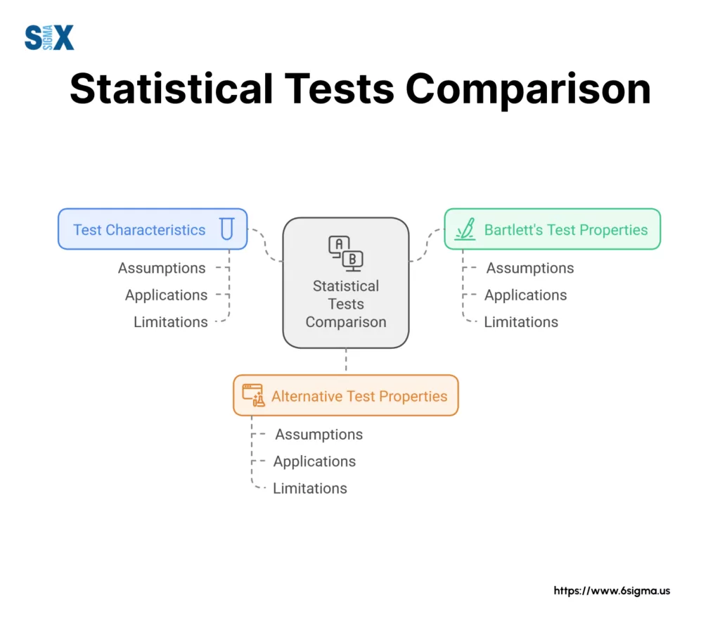
Statistical analysis offers various methods for testing variance homogeneity, each with distinct characteristics and applications.

Understanding these differences enables researchers to select the most appropriate test for their data.

Comparison With Levene’s Test

While Bartlett’s test and Levene’s test both examine variance homogeneity, they differ in key aspects.

Bartlett’s test demonstrates higher statistical power when data follows a normal distribution. However, Levene’s test proves more robust against departures from normality.

The choice between these tests often depends on data characteristics.

Levene’s test maintains reliability even with non-normal distributions, making it preferable for datasets where normality remains uncertain.

Bartlett’s test excels when working with normally distributed data, providing more sensitive detection of variance differences.

Relationship of Bartlett’s Test With ANOVA

Bartlett’s test serves as a preliminary check before conducting ANOVA, rather than an alternative to it.

ANOVA examines mean differences between groups, while Bartlett’s test specifically addresses variance equality.

This relationship positions Bartlett’s test as a diagnostic tool that validates ANOVA’s assumptions rather than a standalone analysis method.

Selection Criteria

The decision to use Bartlett’s test depends on several factors:

• Data normality: Choose Bartlett’s test for normally distributed data
• Sample size equality: Bartlett’s test performs better with equal group sizes
• Research objectives: Select based on whether variance testing serves as a preliminary check or primary analysis
• Field standards: Consider discipline-specific preferences and requirements

This systematic comparison helps researchers make informed decisions about test selection, ensuring appropriate statistical analysis for their specific research contexts.

Bartlett’s Test of Sphericity

Bartlett’s test of sphericity examines whether variables in a dataset are uncorrelated, making it essential for multivariate statistical analyses.

This version of Bartlett’s test differs from the variance homogeneity test, focusing instead on correlation patterns within data matrices.

Definition and Purpose

The sphericity test evaluates whether a correlation matrix resembles an identity matrix.

When variables show no correlation, the population correlation matrix contains ones on the diagonal and zeros elsewhere.

This test proves crucial before conducting factor analysis or principal component analysis, as it determines whether data reduction techniques would yield meaningful results.

Applications of Bartlett’s Test in Factor Analysis

Factor analysis requires sufficient correlation between variables to produce meaningful factors.

The Bartlett sphericity test provides statistical evidence for these correlations.

A significant result (p < 0.05) indicates that variables exhibit sufficient correlation for factor analysis.

In practical applications, researchers use this test to validate their sampling adequacy.

For example, in psychological scale development, the sphericity test helps determine whether questionnaire items measure related constructs.

This statistical procedure maintains particular relevance in fields requiring dimension reduction and scale validation, such as psychometrics and social sciences research.

Conclusion and Future Trends

Bartlett’s test remains a fundamental tool in statistical analysis, providing crucial insights into variance homogeneity across multiple groups.

Its applications span various fields, from traditional research settings to modern data science applications.

Key Statistical Implications

The test continues to serve as a critical prerequisite for many statistical procedures, particularly in experimental design and analysis of variance.

Its role in validating assumptions ensures the reliability of subsequent statistical analyses and research conclusions.

Emerging Applications of Bartlett’s Test

Modern data science and machine learning frameworks incorporate Bartlett’s test in innovative ways.

Automated statistical pipelines now utilize this test for preliminary data assessment, while machine learning algorithms employ it for feature selection and validation procedures.

Future Developments

The evolution of statistical computing suggests new directions for variance testing.

Emerging trends point toward integrated testing frameworks that combine traditional methods with modern computational approaches.

These developments promise enhanced efficiency and accuracy in detecting variance heterogeneity across increasingly complex datasets.

The continued relevance of Bartlett’s test in both classical statistics and modern data analysis underscores its enduring value in the statistical toolkit.

As data science advances, this fundamental test adapts to meet new analytical challenges while maintaining its essential role in statistical methodology.