Articles

Scientists, engineers, and business people need to understand what kind of patterns their data follows.

The normal distribution is one of the most common. But before using techniques that assume normal patterns, it’s good to check if the data matches the normal distribution shape.

The Anderson-Darling normality test is a useful tool for checking how well data fits with the normal distribution.

The Anderson-Darling test gives a number showing how much a data set deviates from the normal distribution shape. This lets researchers decide if normal theory should be used in their data analysis or not.

Key Highlights

• Anderson-Darling normality test examines datasets checking if they follow special patterns.
• Most often it’s checking for normal distribution matching. This normality test helps decide if data significantly diverges from normalcy’s form.
• It provides a detailed measure showing how close data aligns with predicted distribution models, usually normal distribution.
• Wide use exists among quality controllers, production supervisors, and distribution supervisors trying patterns correctly.
• Overall it prevents faulty assumptions misdirecting efforts.

What is the Anderson-Darling Normality Test?

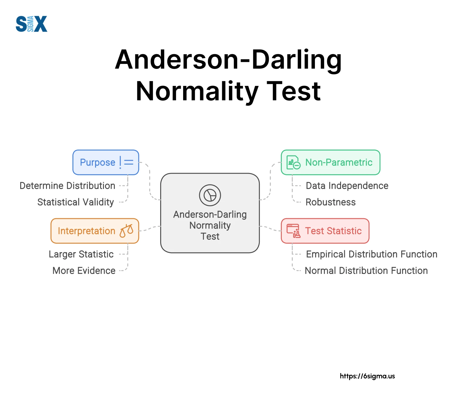
Anderson-Darling normality test checks whether datasets follow certain patterns, especially the normal distribution shape.

It was created by Theodore W. Anderson and Donald A. Darling in 1952 to assess how much a data set matches the normal distribution shape.

The test has become very popular for checking normality properly, especially toward the edges of distributions.

It calculates a statistic judging divergence between the observed info and assumed distribution. Usually, it’s sized up against the normal distribution.

The Anderson-Darling statistic builds upon the Kolmogorov-Smirnov test, emphasizing deviations toward distributions’ ends more sensitively.

This makes it adept at detecting tail differences, an edge propelling its prevalence across sampling sizes and applications from manufacturing to healthcare.

Importance of Normality Testing

Normality testing is a crucial step in many statistical analyses and applications. The assumption of normality is a prerequisite for numerous parametric tests, such as t-tests, ANOVA, and regression analysis. Violating the normality assumption can lead to invalid conclusions and unreliable results.

Moreover, many natural phenomena and processes are assumed to follow a normal distribution, making normality testing essential in various fields, including manufacturing, finance, biology, and physics.

By verifying the normality assumption, researchers and practitioners can make informed decisions and draw accurate inferences from their data.

Advantages of the Anderson-Darling Normality Test

The Anderson-Darling test offers several advantages over other normality tests, such as the Kolmogorov-Smirnov test and the Shapiro-Wilk test:

1. Increased sensitivity: The Anderson-Darling test is more sensitive to deviations from normality, especially in the tails of the distribution, making it better suited for detecting non-normal distributions.
2. Versatility: The test can be applied to complete samples or truncated data, allowing for greater flexibility in data analysis.
3. Efficiency: The Anderson-Darling test is efficient for detecting various types of non-normal distributions, including skewed, heavy-tailed, and bimodal distributions.
4. Ease of interpretation: The test provides a clear decision criterion based on the calculated test statistic and the corresponding critical values or p-value, facilitating a straightforward interpretation of the results.

By utilizing the Anderson-Darling normality test, researchers and practitioners can make informed decisions about the appropriateness of parametric tests and ensure the validity of their statistical analyses.

Background of Anderson-Darling Normality Test

The Anderson-Darling normality test is a statistical procedure used to determine whether a given data set follows a specified probability distribution, such as the normal distribution.

It falls under the category of normality tests, which are essential tools in many areas of statistics and data analysis.

In the context of normality testing, the hypothesis being tested is whether the sample data comes from a normally distributed population.

The null hypothesis (H0) states that the data follows a normal distribution, while the alternative hypothesis (H1) suggests that the data deviates from normality.

Hypothesis testing for normality involves calculating a test statistic and comparing it to a critical value or computing a p-value.

If the test statistic exceeds the critical value or if the p-value is below the chosen significance level (typically 0.05), the null hypothesis of normality is rejected, indicating that the data is unlikely to be normally distributed.

Anderson-Darling Normality Test Statistic

The Anderson-Darling normality test statistic is a measure of the distance between the empirical distribution function (EDF) of the sample data and the cumulative distribution function (CDF) of the hypothesized distribution, in this case, the normal distribution.

The Anderson-Darling test statistic is calculated using the following formula:

A^2 = -n – (1/n) * Σ[(2i-1) * (ln(F(y_i)) + ln(1-F(y_(n+1-i))))]

Where:

• n is the sample size
• y_i are the ordered data points
• F(y_i) is the cumulative distribution function of the hypothesized distribution evaluated at y_i

The Anderson-Darling test statistic gives more weight to the tails of the distribution compared to other normality tests, making it more sensitive to deviations from normality in the tails.

Critical values and p-value calculation

To determine whether the null hypothesis of normality should be rejected or not, the calculated Anderson-Darling normality test statistic is compared to critical values or a p-value is computed.

Critical values for the Anderson-Darling test are tabulated and depend on the sample size and the chosen significance level (e.g., 0.05 or 0.01). If the test statistic exceeds the critical value, the null hypothesis of normality is rejected.

Alternatively, a p-value can be calculated, which represents the probability of observing a test statistic as extreme or more extreme than the calculated value, assuming the null hypothesis is true. If the p-value is less than the chosen significance level, the null hypothesis of normality is rejected.

The p-value for the Anderson-Darling test can be computed using various methods, such as interpolation from tabulated values, approximation formulas, or Monte Carlo simulations.

By comparing the test statistic or p-value to the chosen significance level, researchers can make a decision about whether to reject or fail to reject the null hypothesis of normality for the given data set.

Assumptions and Requirements of the Anderson-Darling Normality Test

The Anderson-Darling normality test, like other statistical tests, has certain assumptions and requirements that must be met for the results to be valid. Understanding these assumptions is crucial to ensure proper application and interpretation of the test.

Sample size considerations

The sample size plays a significant role in the performance of the Anderson-Darling normality test. While there is no strict lower limit on the sample size, the test is generally recommended for moderate to large sample sizes (e.g., greater than 20 observations).

With very small sample sizes, the test may have reduced power to detect deviations from normality.

However, it is important to note that the Anderson-Darling test is more powerful than some other normality tests, such as the Kolmogorov-Smirnov test, for small to moderate sample sizes.

Data requirements

The Anderson-Darling normality test requires a single continuous variable or a set of independent and identically distributed (i.i.d.) observations.

The data should be numerical and measured on at least an interval scale. Categorical or ordinal data cannot be directly tested for normality using the Anderson-Darling normality test.

Normality assumption

The Anderson-Darling normality test is specifically designed to assess whether a given set of data follows a normal (or Gaussian) distribution.

It tests the null hypothesis that the data comes from a normal population against the alternative hypothesis that the data does not follow a normal distribution.

If the normality assumption is violated, the test results may be invalid, and alternative methods for analyzing non-normal data may be required.

It is important to note that the Anderson-Darling test assumes that the parameters of the normal distribution (mean and standard deviation) are unknown and must be estimated from the sample data.

This assumption distinguishes it from other normality tests, such as the Kolmogorov-Smirnov test, which assumes that the parameters are known.

Performing the Anderson-Darling Normality Test

The Anderson-Darling normality test for normality can be performed manually by following these steps:

1. Arrange the data in ascending order: x(1), x(2), …, x(n).
2. Calculate the sample mean and standard deviation.
3. Standardize the data using the formula: (x(i) – sample mean) / sample standard deviation.
4. Calculate the normal scores for each standardized data point using the inverse cumulative distribution function of the standard normal distribution.
5. Calculate the Anderson-Darling normality test statistic using the formula:
   
   A^2 = -n – (1/n) * Sum[(2i – 1) * (ln(Φ(x(i))) + ln(1 – Φ(x(n+1-i)))]
   
   where n is the sample size, Φ is the cumulative distribution function of the standard normal distribution, and x(i) are the ordered data points.

6. Compare the calculated A^2 value with the critical value from the Anderson-Darling table for the chosen significance level (e.g., 0.05). If A^2 exceeds the critical value, reject the null hypothesis that the data follows a normal distribution.

While manual calculation is possible, it can be tedious and error-prone, especially for larger sample sizes.

Using software (Excel, Minitab, R, Python)

Most statistical software packages provide built-in functions or tools to perform the Anderson-Darling normality test with just a few clicks or lines of code. This eliminates the need for manual calculations and reduces the risk of errors.

Excel: The NORM.DIST function can be used to calculate the normal scores, and then the Anderson-Darling statistic can be computed using the formula. However, Excel does not provide a built-in function for the critical values, so you may need to refer to published tables or use an add-in.

Minitab: Minitab offers a dedicated menu option for the Anderson-Darling normality test under the “Stat > Basic Statistics > Normality Test” menu. It provides the test statistic, p-value, and a graphical display of the results.

R: The “nortest” package in R includes the “ad.test” function, which performs the Anderson-Darling normality test and returns the test statistic, p-value, and other relevant information.

Python: The “scipy.stats” module in Python provides the “Anderson” function, which calculates the Anderson-Darling normality test statistic and critical values for a given significance level.

Using software simplifies the process and ensures accurate calculations, especially for larger datasets or when performing multiple tests.

Interpreting results

The interpretation of the Anderson-Darling test results depends on the test statistic (A^2) and the chosen significance level (α, typically 0.05).

1. Calculate the p-value associated with the test statistic. The p-value represents the probability of observing a test statistic as extreme as or more extreme than the calculated value, assuming the null hypothesis (data follows a normal distribution) is true.
2. Compare the p-value with the chosen significance level (α):
   1. If the p-value is less than α, reject the null hypothesis. This suggests that the data does not follow a normal distribution at the given significance level.
   2. If the p-value is greater than or equal to α, fail to reject the null hypothesis. This indicates that there is insufficient evidence to conclude that the data deviates from a normal distribution.
3. Alternatively, compare the test statistic (A^2) with the critical value from the Anderson-Darling table for the chosen significance level:
   1. If A^2 exceeds the critical value, reject the null hypothesis, suggesting that the data is not normally distributed.
   2. If A^2 is less than or equal to the critical value, fail to reject the null hypothesis, indicating that the data is consistent with a normal distribution.

It’s important to note that the Anderson-Darling normality test has higher power than some other normality tests, particularly for detecting deviations from normality in the tails of the distribution.

However, like any statistical test, the results should be interpreted in the context of the specific application and data characteristics.

Comparison with Other Normality Tests

The Anderson-Darling normality test is one of several statistical tests used to assess whether a sample of data follows a normal distribution. It’s important to understand how it compares to other popular normality tests in terms of strengths, limitations, and appropriate use cases.

Anderson-Darling Normality Test vs. Shapiro-Wilk

The Shapiro-Wilk test is another widely used normality test, especially for smaller sample sizes (n<50). Like the Anderson-Darling, it tests the null hypothesis that a sample came from a normally distributed population. Both tests are more powerful than older tests like the Kolmogorov-Smirnov for detecting departures from normality.

The key difference is that the Shapiro-Wilk test tends to be better at detecting departures from normality due to outliers, while the Anderson-Darling normality test is more sensitive to discrepancies in the tails of distributions.

For samples from non-normal distributions with short tails, the Shapiro-Wilk may be preferred. But for heavier-tailed distributions, the Anderson-Darling normality test is generally considered superior.

Anderson-Darling Normality Test vs. Kolmogorov-Smirnov

The Kolmogorov-Smirnov (K-S) test was one of the first goodness-of-fit tests for normality. It quantifies the maximum distance between the empirical distribution function and the cumulative normal distribution. 

While the K-S test is easy to calculate and understand, it tends to be less powerful than more modern tests like Anderson-Darling normality test and Shapiro-Wilk at detecting deviations from normality, especially in the tails. The Anderson-Darling test places more emphasis on the tails than the K-S test.

For very large sample sizes (n>2000), the K-S may be preferred due to the difficulties in calculating critical values for the Anderson-Darling distribution. But for most practical applications with smaller to moderate samples, Anderson-Darling is favored.

Strengths and Limitations of Anderson-Darling Normality Test

The Anderson-Darling test has several key strengths:

• It is a powerful test for detecting many types of non-normal distributions
• It gives more weight to the tails than the K-S test, making it sensitive to outliers
• Critical values are widely available for a range of sample sizes
• It makes use of the specific distribution being tested (normal, lognormal, etc.)

However, some limitations include:

• For very small samples (n<8), other tests may be preferred
• For very large samples (n>2000), calculating critical values becomes difficult
• Like all tests, it has reduced power for certain alternative distributions
• The assumptions of randomness and continuity must be met

Overall, the Anderson-Darling is an excellent general-purpose option for normality testing across many fields when the sample is not extremely large or small. Understanding how it compares to other tests is important for proper application and interpretation.

Applications of the Anderson-Darling Normality Test

Quality control and process monitoring

The Anderson-Darling normality test finds extensive applications in quality control and process monitoring. In manufacturing and production environments, it is crucial to ensure that the processes are operating within specified limits and producing outputs that conform to quality standards.

The Anderson-Darling test can be used to verify the normality assumption of the process data, which is a common requirement for many statistical process control (SPC) techniques, such as control charts.

By checking the normality of process data, manufacturers can detect deviations from the expected distribution, which may indicate the presence of assignable causes or special causes of variation.

This information can then be used to take corrective actions and bring the process back into a state of statistical control, ultimately improving product quality and reducing waste.

Distribution fitting

Another important application of the Anderson-Darling test is in distribution fitting. Many statistical models and analyses assume that the underlying data follows a specific probability distribution, such as the normal, exponential, or Weibull distribution.

The Anderson-Darling test can be used to assess the goodness-of-fit of the data to these theoretical distributions.

By determining the most appropriate distribution for the data, analysts can make more accurate inferences, predictions, and decisions.

For example, in reliability engineering, the Anderson-Darling test can be used to fit a Weibull distribution to failure time data, which can then be used to estimate the reliability of a product or system.

Goodness-of-fit testing

Closely related to distribution fitting is the use of the Anderson-Darling test for goodness-of-fit testing. In this context, the test is used to evaluate whether a sample of data follows a hypothesized distribution, such as the normal or exponential distribution.

This is particularly important in fields like finance, where the assumption of normality is often made for asset returns or risk models.

By performing goodness-of-fit tests, researchers and analysts can validate the assumptions underlying their statistical models and ensure that the chosen distribution is appropriate for the data at hand.

If the data does not follow the assumed distribution, alternative models or transformations may need to be considered.

Case Studies and Examples

To illustrate the practical applications of the Anderson-Darling normality test, let’s consider a few real-world examples:

1. Quality control in semiconductor manufacturing: In the semiconductor industry, the thickness of thin-film layers is a critical quality characteristic.
   
   The Anderson-Darling test can be used to verify the normality assumption of the thickness measurements, which is necessary for implementing effective statistical process control techniques.
   
2. Reliability analysis of wind turbines: In the renewable energy sector, the Anderson-Darling test can be used to assess the goodness-of-fit of wind speed data to a Weibull distribution.
   
   This information is crucial for estimating the power output and reliability of wind turbines.
   
3. Financial risk modeling: In finance, many risk models, such as Value-at-Risk (VaR) calculations, assume that asset returns follow a normal distribution.
   
   The Anderson-Darling test can be used to validate this assumption and ensure the accuracy of risk estimates.
   
4. Environmental data analysis: In environmental studies, the Anderson-Darling test can be applied to various data sets, such as pollutant concentrations or meteorological measurements, to determine if they conform to specific theoretical distributions.
   
   This information can aid in modeling and decision-making processes related to environmental management and policy.

These examples illustrate the versatility and practical relevance of the Anderson-Darling normality test across various industries and domains, highlighting its importance as a fundamental tool in statistical analysis and decision-making.

Additional Resource

Many statistical software packages include built-in functions or modules for performing the Anderson-Darling normality test. These packages offer a convenient way to conduct the test and often provide additional features and visualizations.

In Excel, the Anderson-Darling test can be performed using add-ins or user-defined functions. One popular add-in is the SPC XL Add-in, which includes an Anderson-Darling normality test function.

Minitab, a widely used statistical software, has a dedicated function for the Anderson-Darling test. The “ANDDARLING” function in Minitab calculates the test statistic and p-value, making it easy to perform the test and interpret the results.

For users of the R programming language, the “nortest” package provides a comprehensive set of tools for normality testing, including the Anderson-Darling test. The “ad.test” function in this package allows you to perform the test and obtain the test statistic and p-value.

Similarly, in Python, the “scipy.stats” module offers the “anderson” function, which calculates the Anderson-Darling test statistic and critical values for a given data set.

These software packages often provide additional features, such as graphical representations, hypothesis testing, and integration with other statistical analyses, making them valuable tools for conducting the Anderson-Darling normality test and interpreting the results.