Right-Skewed Histogram: A Master Black Belt’s Guide to Asymmetric Data Analysis
Approximately 70% of real-world data distributions do not follow the typical bell curve.
It is especially common in finance and business to find histograms that are right-skewed, but these histograms are often misunderstood.
By the end of this article, you’ll understand
- The definition and characteristics of right-skewed histograms
- How to identify and interpret the right skewness in your data
- The mathematical foundations, including variance and standard deviation
- Real-world applications across various industries
- Advanced techniques for handling right-skewed data
A six sigma certification can take your understanding further, equipping you to apply these concepts in process improvement.
Let’s embark on this journey to transform how you view and analyze asymmetric data distributions.
What is a Right Skewed Histogram?
Right-skewed histograms also called positively skewed histograms, are fundamental concepts in statistics.
Right-skewed histograms asymmetrically display data, with the tail of the distribution extending towards the right side, resulting in most data points located on the left side and a few located on the right side.
Understanding right-skewed histograms is fundamental for data analysis. Earning a six sigma certification can help you master these concepts and apply them to optimize processes.
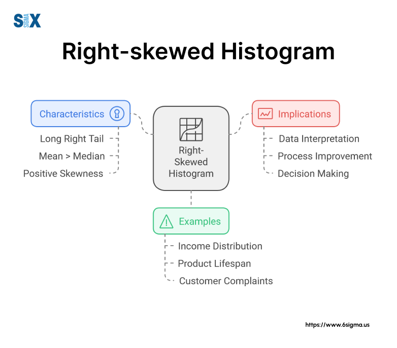
Key characteristics and properties of a right-skewed histogram include:
- Longer tail on the right side
- Peak (mode) closer to the left side
- The mean is typically greater than the median, which is greater than the mode
- Asymmetrical shape
Curious about the basics? Our Six Sigma White Belt certification course offers an easy entry into statistical analysis and Six Sigma concepts.
Ready to deepen your understanding of data distributions?
Our Lean Six Sigma Green Belt course covers this and more. Get comprehensive training on statistical analysis techniques.
Identifying Right-Skewed Distributions
Recognizing the right skewness in your data is crucial for proper analysis and interpretation. Here’s a step-by-step guide to spotting the right skewness:
- Visualize the data: Create a histogram or box plot of your data.
- Observe the tail: Look for a longer tail extending to the right.
- Locate the peak: Check if the highest point (mode) is on the left side.
- Compare mean and median: Calculate these measures; in right-skewed distributions, the mean is typically greater than the median.
Common misconceptions about right-skewed histograms include
- Assuming all asymmetric distributions are right-skewed
- Confusing right skewness with outliers
- Overlooking the impact of sample size on skewness
Understanding right-skewed histograms is essential for accurate data interpretation in various fields, from finance to quality control. In my work with companies like 3M and Dell, recognizing the right skewness has been crucial in identifying process inefficiencies and optimizing production systems.
The Mathematics Behind a Right Skewed Histogram
As a Six Sigma Master Black Belt, I’ve learned that understanding the mathematical underpinnings of right-skewed histograms is crucial for accurate data interpretation and decision-making.
Let’s dive into the key mathematical concepts that define these distributions.
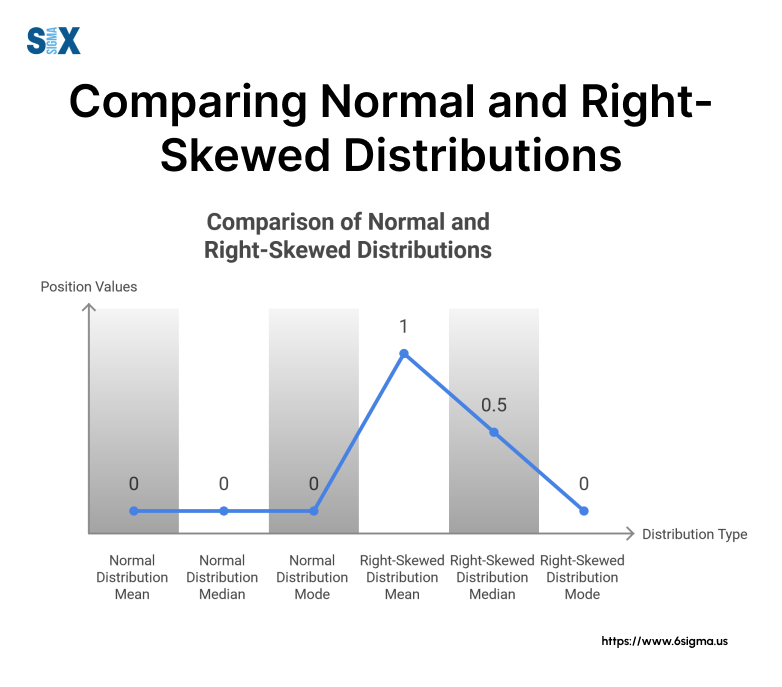
Mean, Median, and Mode Relationships
In a right-skewed histogram, the relationship between the mean, median, and mode is distinct from that of a normal distribution. Here’s what you need to know:
- Mean > Median > Mode
- The mean is pulled towards the tail (right side) due to extreme values
- The median is less affected by outliers and sits between the mean and mode
- The mode represents the peak of the distribution, located on the left side
This unique relationship is vital for describing a right-skewed histogram accurately. For instance, in a project, we analyzed customer complaint data that showed this pattern.
Understanding the mean-median-mode relationship helped us identify the most common issues (mode) while also considering the impact of severe, less frequent problems (reflected in the mean).
In Six Sigma, grasping these mathematical relationships is key to data-driven decisions. A six sigma certification provides the tools to analyze skewed distributions accurately.
Measures of Skewness
To quantify the degree of right skewness, we use skewness coefficients. The most common are:
- Pearson’s First Coefficient of Skewness: (Mean – Mode) / Standard Deviation
- Pearson’s Second Coefficient of Skewness: 3(Mean – Median) / Standard Deviation
Practical interpretation of skewness values
- Values close to 0 indicate symmetry
- Positive values indicate right skewness
- The larger the positive value, the more pronounced the right skew
We used these coefficients to compare process outputs across different manufacturing lines, allowing us to standardize our improvement efforts.
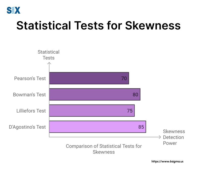
Statistical Tests for Skewness
To formally test for skewness, we often employ statistical tests. Common tests include
- D’Agostino’s K-squared test
- Jarque-Bera test
- Anderson-Darling test
When to apply these tests
- To confirm visual observations of skewness
- When deciding between parametric and non-parametric statistical methods
- In quality control, to detect shifts in process distribution
- Formulate hypotheses (H0: Distribution is not skewed, H1: Distribution is skewed)
- Choose a significance level (typically 0.05)
- Calculate test statistic
- Compare the pare p-value to the significance level
- Draw conclusion
- Natural Limitations
- Minimum Values: Many variables have a natural lower bound but no upper limit. For example, in a project I led, we analyzed customer wait times. The minimum time was zero, but there was no theoretical maximum, leading to right skewness.
- Maximum Effort: In performance metrics, there’s often a ceiling effect where most performers cluster near the top, with a few lagging behind, creating the right skewness.
- Sampling Biases and Errors
- Selection Bias: If sampling methods favor certain groups, it can lead to right skewness. In a healthcare project, we initially saw right-skewed patient satisfaction scores due to the under-representation of critically ill patients.
- Measurement Errors: Systematic errors in data collection can create artificial skewness. We once discovered this in a manufacturing process where faulty sensors were underreporting high values.
- Challenges in Using Standard Statistical Methods
- Many statistical tests assume normality, which right-skewed data violates.
- Measures like mean and standard deviation can be misleading in right-skewed distributions.
- Importance in Decision-Making
- Ignoring skewness can lead to flawed conclusions. In a supply chain project, recognizing right skewness in delivery times helped us set more realistic performance targets.
- Right skewness often indicates the presence of high-impact, low-frequency events that require special attention.
- Right-skewed data can be easily misrepresented, intentionally or unintentionally, leading to incorrect conclusions.
- In financial reporting, for instance, using only mean values for right-skewed profit distributions can paint an overly optimistic picture.
- Always provide multiple measures of central tendency (mean, median, mode) for right-skewed data.
- Use visual representations that clearly show the skewness.
- Explain the implications of skewness in your analysis to stakeholders.
- One of the most classic examples of a right-skewed histogram is income distribution. During a project with a major retail chain, we analyzed employee salary data.
- The histogram revealed a pronounced right skew, with a large number of entry-level and mid-range salaries clustering on the left, and a long tail stretching to the right representing higher-paid executives and specialists.
- This right-skewed histogram meaning became crucial in developing fair compensation strategies and identifying potential wage gaps.
- In a consulting project for a financial services firm, we examined daily stock returns.
- The histogram of returns typically showed a right skew, with most returns clustered around a small positive value, but with occasional large positive returns creating a long right tail.
- Understanding this skew was essential for accurate risk assessment and portfolio management.
- While working with an environmental agency, we analyzed air quality data. The histogram of particulate matter concentrations often displayed right skewness.
- Most days had relatively low levels, but occasional spikes due to factors like wildfires or industrial accidents created a long right tail.
- This pattern helped in setting appropriate air quality standards and developing emergency response plans.
- In a biodiversity study, the histogram of species abundance often showed right skewness.
- Many species were represented by a few individuals, while a few species were highly abundant, creating a classic right-skewed pattern.
- This insight was crucial for conservation efforts and understanding ecosystem health.
- During an educational consulting project, we frequently encountered right-skewed histograms in standardized test scores.
- Most students scored in the middle range, with fewer high-achieving outliers creating a tail to the right.
- Recognizing this pattern was vital for fair grading practices and identifying gifted students.
- In a digital marketing project for a tech company, we analyzed social media engagement data.
- The histogram of likes, shares, and comments often showed extreme right skewness, with most posts getting modest engagement and a few “viral” posts creating a long right tail.
- This insight guided content strategy and performance benchmarking.
- In a hospital efficiency project, patient wait times often form a right-skewed histogram.
- Most patients were seen relatively quickly, but complex cases led to occasional long waits, creating a right skew.
- Understanding this pattern was crucial for improving patient flow and resource allocation.
- In a quality control project for a manufacturing client, we observed that defect rates often followed a right-skewed distribution.
- Right-skewed defect rates signal variability. Root cause analysis training can help you pinpoint and fix the underlying issues.
- Most production runs had few defects, but occasional problematic batches created a long right tail.
- This insight guided our Six Sigma improvement efforts, focusing on reducing variability and eliminating high-defect outliers.
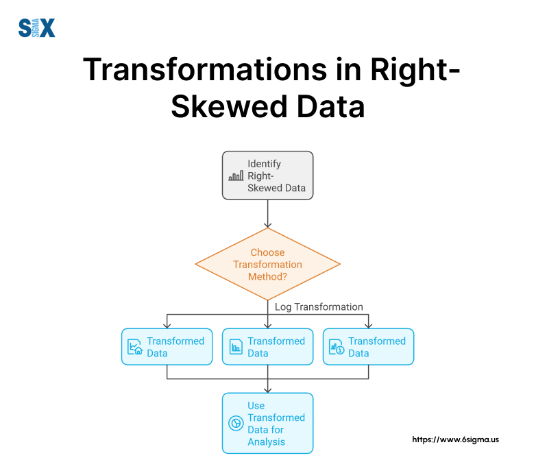
- Logarithmic and Other Common Transformations
- Logarithmic transformation: Often the go-to choice for right-skewed data
- Square root transformation: Useful for less severe skewness
- Inverse transformation: Effective for certain types of right-skewed data
- When and How to Apply Transformations
- Use transformations when assumptions of normality are violated
- Always plot the transformed data to ensure it achieves the desired effect
- Be cautious about interpreting results in the transformed scale
- Identification of True Outliers vs. Expected Extremes
- Use statistical methods like the Interquartile Range (IQR) method
- Consider domain knowledge to distinguish between true outliers and expected extreme values
- Techniques for Managing Outliers Without Data Loss
- Winsorization: Capping extreme values at a specified percentile
- Robust statistical methods that are less sensitive to outliers
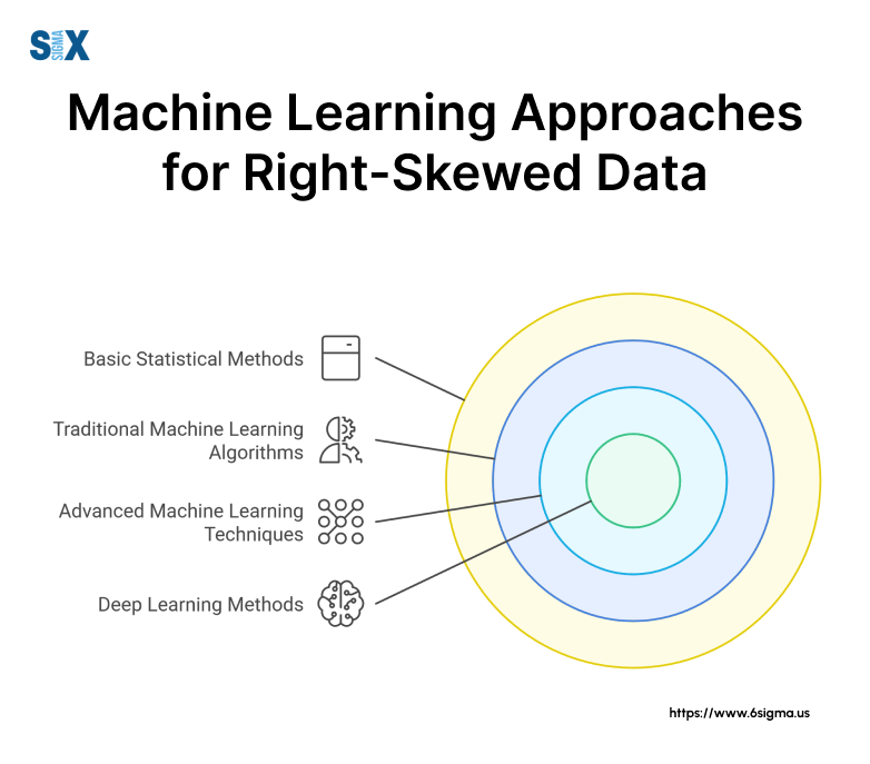
- Algorithms Suited for Skewed Data
- Decision trees and random forests are often robust to skewness
- Gradient boosting algorithms can handle non-linear relationships in skewed data
- Future Trends in Handling Asymmetric Distributions
- Automated feature engineering to handle skewness
- Ensemble methods that combine multiple approaches for skewed data
- Data Collection Considerations
- Ensure your sample size is large enough to detect skewness accurately
- Be aware of potential sources of bias that could artificially create or mask skewness
- Use consistent measurement techniques to avoid introducing errors
- Exploratory Data Analysis Techniques
- Start with basic descriptive statistics (mean, median, mode, range)
- Create a histogram to visually assess the distribution
- Calculate the skewness coefficient to quantify the degree of right skew
- Use box plots to identify potential outliers
- Choosing Appropriate Statistical Methods
- For slightly right-skewed histograms, standard parametric tests may still be applicable
- For more pronounced skewness, consider non-parametric tests or data transformations
- Always check the assumptions of your chosen statistical method
- Effective Histogram Creation
- Choose an appropriate number of bins (too few or too many can obscure the distribution)
- Use consistent bin widths unless there’s a compelling reason not to
- Consider using relative frequency on the y-axis for easier comparison across datasets
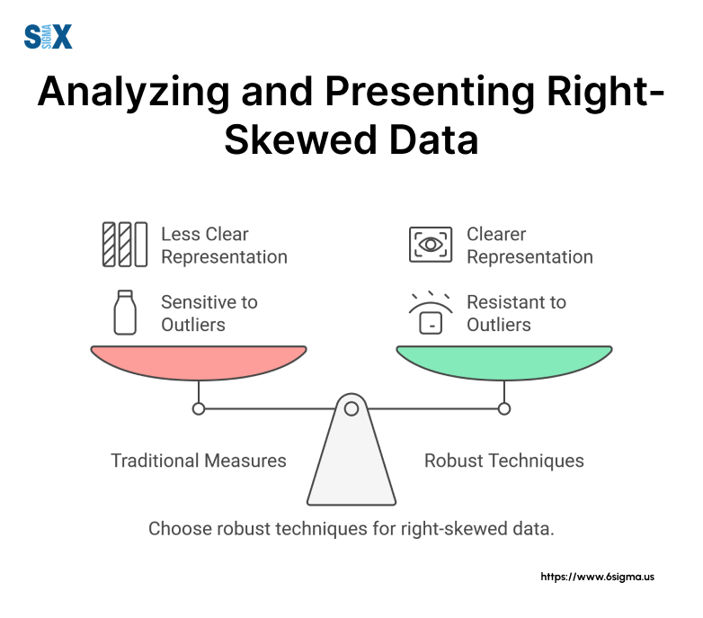
- Alternative Visualization Methods for Skewed Data
- Q-Q plots to compare your data against a normal distribution
- Box plots to show the median and quartiles while highlighting outliers
- Violin plots combine aspects of box plots with density plots
- Tips for Clear and Accurate Presentation
- Always include a visual representation of the data alongside numeric summaries
- Report both mean and median, explaining the difference in right-skewed contexts
- Use clear, jargon-free language to describe the skewness and its implications
- Addressing Potential Misinterpretations
- Explain why traditional measures like mean might be misleading
- Discuss the impact of outliers on your analysis
- Provide context for why the skewness occurs in your data
- Key Figures and Their Contributions
- Karl Pearson (1857-1936): Introduced the concept of “skewness” in 1895
- Ronald Fisher (1890-1962): Developed measures of skewness in the 1920s
- John Tukey (1915-2000): Pioneered exploratory data analysis techniques that highlighted the importance of understanding skewed distributions
- Evolution of Understanding and Analysis Methods
- Early 20th century: Focus on mathematical definitions and properties of skewed distributions
- Mid-20th century: Development of robust statistical methods to handle non-normal data
- Late 20th century: Increased emphasis on graphical representations and computer-assisted analysis of skewed data
- Recent Developments in Handling Skewed Data
- Advanced computational methods for modeling complex, skewed distributions
- Machine learning algorithms that can automatically detect and adapt to data skewness
- Bayesian approaches that incorporate prior knowledge about data asymmetry
- Emerging Challenges and Research Areas
- Big data analytics: Handling skewness in extremely large datasets
- Multi-dimensional skewness: Extending concepts to high-dimensional data
- Causal inference with skewed data: Understanding how skewness affects causal relationships
- The distinctive shape and characteristics of right-skewed histograms
- The importance of recognizing skewness in data analysis and decision-making
- Practical techniques for handling and interpreting right-skewed data
- Advanced methods for transforming and analyzing skewed distributions
How to apply
During a project, we used D’Agostino’s K-squared test to validate our initial observations of right skewness in product defect rates, which guided our subsequent process improvement strategies.
Understanding these mathematical concepts allows for more precise analysis and description of right-skewed histograms, leading to better-informed decisions in various business contexts.
Causes and Implications of a Right Skewed Histogram
As a Six Sigma Master Black Belt with extensive experience across various industries, I’ve encountered numerous instances of right-skewed histograms.
Understanding what causes right skewness and its implications is crucial for accurate data interpretation and decision-making. Let’s explore this topic in depth.
Common Causes in Data Collection
Right skewness often emerges due to natural limitations or biases in data collection processes. Common causes include:
Implications of a Right Skewed Histogram for Data Analysis
Recognizing the right skewness is vital for several reasons:
Ethical Considerations
As data professionals, we have an ethical responsibility to accurately represent and interpret data:
Potential for Misinterpretation
Best Practices for Reporting Skewed Data
Understanding the causes and implications of right skewness is crucial for anyone working with data. It enables more accurate analysis, better decision-making, and ethical reporting of results.
Recognizing skewness is vital for effective decision-making. With a six sigma certification, you’ll be trained to spot and address these patterns in any industry.
Examples and Applications of a Right Skewed Histogram
I’ve encountered numerous applications of right-skewed histograms across various industries.
Understanding these examples can help you recognize when to use right-skewed histograms in your work. Let’s explore some case studies and applications.
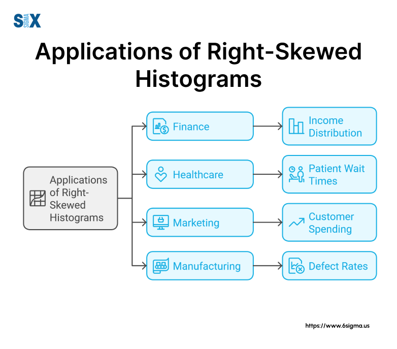
Economic and Financial Data
Income Distribution Case Study
Stock Market Returns Analysis
Natural and Environmental Sciences
Pollution Levels Example
Species Distribution Patterns
Social Sciences and Psychology
Test Scores Distribution:
Social Media Engagement Metrics
Interdisciplinary Applications
Healthcare Wait Times
Manufacturing Defect Rates
In manufacturing, right-skewed defect rates are common. A six sigma certification prepares you to analyze these patterns and drive quality improvements.
Want to apply these concepts in real-world scenarios? Our Lean Six Sigma Black Belt program offers advanced training in data analysis and process improvement.
More Topics in a Right Skewed Histogram Analysis
My experience as a Six Sigma Master Black Belt has taught me that mastering these advanced topics can significantly enhance your data analysis capabilities and decision-making processes.
Data Transformations
When dealing with right-skewed data, transformations can be a powerful tool to normalize the distribution and make it more amenable to standard statistical techniques.
In a project with a semiconductor manufacturer, we applied a log transformation to cycle time data, which allowed us to use standard statistical process control techniques effectively.
Handling Outliers in a Right Skewed Histogram
Right-skewed histograms often come with outliers, which can significantly impact analysis if not handled properly.
During a quality improvement project, we used Winsorization to handle extreme values in customer response times, which allowed us to maintain data integrity while mitigating the impact of outliers.
Machine Learning Approaches
As data science evolves, machine learning offers new ways to handle right-skewed data.
In a recent project with a fintech startup, we employed gradient boosting algorithms to predict loan defaults from right-skewed financial data, achieving higher accuracy than traditional methods.
It’s worth noting that while these advanced techniques are powerful, they should be used judiciously. Always start with a thorough understanding of your data and the underlying processes. Sometimes, a right-skewed histogram or a bimodal right-skewed histogram is a natural and important feature of your data that shouldn’t be “corrected” but rather understood and leveraged for insights.
As the field of data science continues to evolve, staying updated on these advanced techniques will be crucial for any professional working with complex, real-world data distributions.
At SixSigma.us, we continuously update our training programs to include these cutting-edge methods, ensuring our clients are always equipped with the latest tools to handle challenging data scenarios.
Stay ahead in data analysis. Our Design for Six Sigma (DFSS) course covers cutting-edge statistical methods and their applications.
Practical Guide: Analyzing and Presenting Right-Skewed Data
I’ve found that knowing how to effectively analyze and present right-skewed data is crucial for making informed decisions.
A structured analysis process is a Six Sigma hallmark. Earning a six sigma certification introduces you to these methods for handling skewed data.
Let’s walk you through the process, from data collection to result presentation, ensuring you can confidently handle right-skewed histograms in your projects.
Step-by-Step Analysis Process
Visualization Best Practices of a Right Skewed Histogram
Reporting and Communicating Results
When describing a right-skewed histogram, be specific about the shape and its implications. For example, in a project I led, we encountered a slightly right-skewed histogram of customer service response times. We described it as follows:
“The distribution of response times shows a slight right skew, with a peak around 5 minutes and a long tail extending to 30 minutes. This indicates that while most inquiries are resolved quickly, a small number of complex cases require significantly more time. The median response time of 6 minutes provides a more representative measure of typical performance than the mean of 8 minutes, which is influenced by the long tail.”
Remember, the goal is not just to identify the skewness, but to understand its implications for your process or system. This understanding is what drives meaningful improvements and informed decision-making in Six Sigma projects and beyond.
Historical Context and Evolution of Skewness Concepts
This historical perspective is crucial for appreciating the depth and importance of these concepts in modern data analysis.
Brief History of Skewness in Statistics
The concept of skewness has a rich history dating back to the early days of statistics:
Current State and Future Directions
The field of statistics continues to evolve, particularly in its approach to skewed data:
I’ve seen how these evolving concepts have transformed the approach to data analysis. For instance, in a recent project analyzing customer satisfaction scores, we employed advanced machine learning techniques to handle the inherent right skew in the data, leading to more accurate predictions and targeted improvement strategies.
Understanding this historical context and staying abreast of current developments is crucial for anyone working with data allows us to appreciate the nuances of right-skewed histograms and choose the most appropriate, cutting-edge methods for analysis.
Conclusion
Understanding these asymmetric distributions is crucial for anyone working with data.
Key takeaways include
Mastering these concepts is not just an academic exercise—it’s a vital skill for driving process improvement and making informed business decisions.
Whether you’re analyzing customer satisfaction scores, financial data, or manufacturing processes, the ability to recognize and work with right-skewed histograms will set you apart as a data-savvy professional.
For those eager to delve deeper, I invite you to explore our advanced courses at SixSigma.us. We offer comprehensive training on statistical analysis and process improvement techniques that build on the concepts we’ve discussed here.
By embracing the complexities of right-skewed histograms and other non-normal distributions, you’ll be better equipped to tackle the challenges of our data-driven world.
SixSigma.us offers both Live Virtual classes as well as Online Self-Paced training. Most option includes access to the same great Master Black Belt instructors that teach our World Class in-person sessions. Sign-up today!
Virtual Classroom Training Programs Self-Paced Online Training Programs